# Light Tunnel Mk2

{% columns %}
{% column %}

<figure><img src="/files/13CXXYbFAbNHcDeETDsS" alt=""><figcaption></figcaption></figure>
{% endcolumn %}

{% column %}
The Light Tunnel produces [**i.i.d.**](#user-content-fn-1)[^1] **data and images** from a controlled **optical experiment.**

It contains a controllable light source, linear polarizers mounted on rotating frames, and sensors to measure light intensity at different frequencies and locations. A camera captures images from inside the tunnel.
{% endcolumn %}
{% endcolumns %}

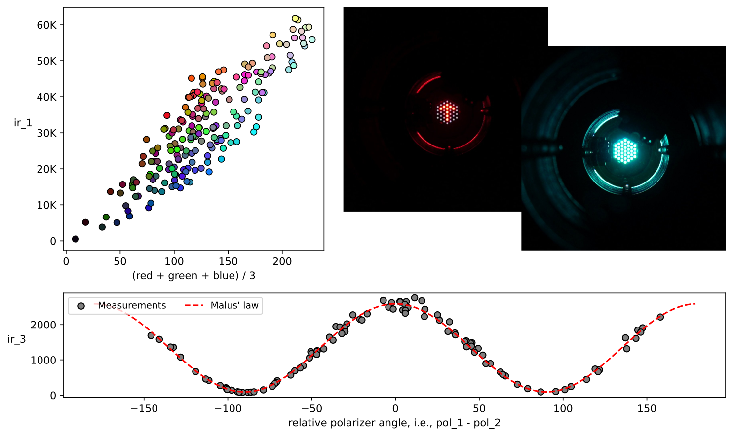
The chamber produces images and i.i.d. data from up to 99 [variables](#variables-table), including sensor measurements, control inputs, and sensor parameters.

<figure><picture><source srcset="/files/i9d1XaXEIWKgu9DpvXqr" media="(prefers-color-scheme: dark)"><img src="/files/TBn5w9odQ0YwZonA3XA7" alt="" width="563"></picture><figcaption><p><strong>Top right</strong>: infrared-intensity measurements produced by the first sensor (<code>ir_1</code>) for different intensities of the light-source channels (<code>red/green/blue</code>). <strong>Top left</strong>: examples of images produced by the tunnel in the linked_leds (left) and the camera_fast (right) <a href="#hardware-configurations">hardware configurations</a>. <strong>Bottom:</strong> observing Malus' law in the effect of the polarizer positions (<code>pol_1, pol_2</code>) on the infrared intensity at the third sensor (<code>ir_3</code>).</p></figcaption></figure>

<details>

<summary>Chamber diagram &#x26; variables</summary>

You can find a description of each variable in the documentation for each [hardware configuration](#hardware-configurations) below.

<figure><img src="/files/8FjeX1grNB9Zz1mh4FBD" alt=""><figcaption><p>Right click to download the image (available under a <a href="https://creativecommons.org/licenses/by-nc/4.0/">CC BY-NC 4.0</a> non-commercial license).</p></figcaption></figure>

</details>

<details>

<summary>Simulators</summary>

See the [Simulator Index](https://github.com/juangamella/causal-chamber-package/tree/main/causalchamber/simulators) for a list of the simulators we offer for this chamber, including documentation and example code.

</details>

### Hardware configurations

Like all chambers, the wind tunnel can automatically load different [hardware configurations](/the-chambers/how-they-work.md#hardware-configurations). See the corresponding PDF for a chamber diagram, a complete description of all variables, and the causal ground-truth graph.

<table><thead><tr><th width="203.956787109375">Name</th><th width="77.6397705078125" data-type="checkbox">Img. data</th><th width="243.657958984375">Description</th><th width="149.1961669921875">Documentation</th><th>Causal ground-truth</th></tr></thead><tbody><tr><td><code>standard</code></td><td>false</td><td>Standard configuration with all variables (no camera).</td><td><a href="https://cchamber-box.s3.eu-central-2.amazonaws.com/config_doc_lt_mk2_standard.pdf" class="button secondary">.pdf</a></td><td><a href="https://box.causalchamber.ai/gt_graph_lt_mk2_standard.pdf" class="button secondary">.pdf</a></td></tr><tr><td><code>linked_leds</code></td><td>false</td><td>Additional tunable causal effects.</td><td><a href="https://cchamber-box.s3.eu-central-2.amazonaws.com/config_doc_lt_mk2_linked_leds.pdf" class="button secondary">.pdf</a></td><td><a href="https://box.causalchamber.ai/gt_graph_lt_mk2_linked_leds.pdf" class="button secondary">.pdf</a></td></tr><tr><td><code>linked_leds_sigmoid</code></td><td>false</td><td>Same as <code>linked_leds</code> but with tunable non-linear effects.</td><td><a href="https://cchamber-box.s3.eu-central-2.amazonaws.com/config_doc_lt_mk2_linked_leds_sigmoid.pdf" class="button secondary">.pdf</a></td><td><a href="https://box.causalchamber.ai/gt_graph_lt_mk2_linked_leds.pdf" class="button secondary">.pdf</a></td></tr><tr><td><code>camera_fast</code></td><td>true</td><td>Provides images and camera variables.</td><td><a href="https://cchamber-box.s3.eu-central-2.amazonaws.com/config_doc_lt_mk2_camera_fast.pdf" class="button secondary">.pdf</a></td><td><a class="button secondary">.pdf</a></td></tr><tr><td><code>led_matrix</code></td><td>true</td><td>Same as <code>camera_fast</code> but with individual control of the light-source LEDs.</td><td><a href="https://cchamber-box.s3.eu-central-2.amazonaws.com/config_doc_lt_mk2_led_matrix.pdf" class="button secondary">.pdf</a></td><td><a class="button secondary">.pdf</a></td></tr></tbody></table>

### Map of effects

Here you can find a detailed description of all effects between chamber variables, together with additional experiments and figures. Throughout, we use an edge A $$\longrightarrow$$ B to denote that a variable A has an effect on variable B.

> **Short-hand notation**
>
> * A1/2 $$\longrightarrow$$ B, C is equivalent to the edges A1 $$\longrightarrow$$ B, A1 $$\longrightarrow$$ C, A2 $$\longrightarrow$$ B and A2 $$\longrightarrow$$ C
> * We can also express this as A\* $$\longrightarrow$$ B,C

Some text and figures in this section are adapted from the [original paper](https://www.nature.com/articles/s42256-024-00964-x) (Gamella et al. 2025, [Appendix III](https://static-content.springer.com/esm/art%3A10.1038%2Fs42256-024-00964-x/MediaObjects/42256_2024_964_MOESM1_ESM.pdf)).

{% hint style="info" %}
Some [hardware configurations](#hardware-configurations) introduce additional effects between variables. See their [documentation](#hardware-configurations) for the complete map of physical effects.
{% endhint %}

{% tabs %}
{% tab title="Graph" %}

<figure><img src="/files/iB6bZdiW4lSaqPJbS5xu" alt=""><figcaption><p>Right click to download the image (available under a <a href="https://creativecommons.org/licenses/by-nc/4.0/">CC BY-NC 4.0</a> non-commercial license).</p></figcaption></figure>
{% endtab %}
{% endtabs %}

<details>

<summary>Disclaimer: causal ground-truth</summary>

The graph above can be interpreted as a **causal ground truth**, as formalized in Gamella et al. (2025, [Appendix V](https://cchamber-box.s3.eu-central-2.amazonaws.com/nature_paper_appendices.pdf)), i.e., an edge X $$\longrightarrow$$ Y signifies that—for some value of the other chamber inputs—an intervention on X will change the distribution of subsequent measurements of Y. The graph should <mark style="color:$danger;">**not**</mark> be taken as a graphical model of statistical dependencies, as [external influences](#external-influences) on the system may create additional correlations between variables.

</details>

In what follows, we provide a detailed description and visualization of each edge (physical effect) in the above graph.

{% hint style="info" %}
See the [variables table](#variables-table) for a description of all variables in this section.
{% endhint %}

***

#### `red`, `green`, `blue` $$\longrightarrow$$ `ir_1/2/3`, `vis_1/2/3`

The brightness settings of the light-source colors (`red`, `green`, `blue`) affect the readings of the three light-intensity sensors. Each sensor produces two measurements: one for the infrared part of the spectrum (`ir_j`), and another for the visible part (`vis_j`). The effect of each color is approximately linear with heteroscedastic noise, and the slope is determined by its [typical wavelength](#user-content-fn-2)[^2] and the sensor's [spectral sensitivity](#user-content-fn-3)[^3].

{% tabs %}
{% tab title="Figure 1" %}

<figure><img src="/files/Ro6AD74msttFxIcmVC6k" alt=""><figcaption><p>Effect of each light-source color—controlled by the variables <code>red</code>, <code>green</code>, <code>blue</code>—on the measurements produced by the three light-intensity sensors <code>ir_1/2/3</code> and <code>vis_1/2/3</code>.  The sensors are placed at increasing distances from the light source (with the first sensor closest to it), resulting in a decrease in the maximum measurement value. The infrared channel (<code>ir_j</code>, top row) of the sensors is most sensitive to red light, whereas the effect is reversed for the visible channel (<code>vis_j</code>, bottom row).</p></figcaption></figure>
{% endtab %}

{% tab title="Experiment" %}
To recreate the data for the figure using the [Remote Lab](/remote-lab/quickstart.md):

{% code overflow="wrap" %}

```python
# Connect to the lab
import causalchamber.lab as lab
rlab = lab.Lab(credentials_file = '.credentials', verbose=False)

# Define experiment
experiment = rlab.new_experiment('lt-aeon-dlpv', 'standard')

rng = np.random.default_rng(42)

N = 300

colors = ['red', 'green', 'blue']

for i,value in zip(rng.choice([0,1,2], size=N), rng.integers(0,256,size=N)):
    # Set flag
    experiment.set('flag', i)
    # Set all colors to zero
    [experiment.set(cc, 0) for cc in colors]
    # Set random color value and take a measurement
    experiment.set(colors[i], value)
    experiment.measure(n=1)

# Submit
eid = experiment.submit(tag='ls-colors')
```

{% endcode %}
{% endtab %}
{% endtabs %}

#### `red`, `green`, `blue` $$\longrightarrow$$ `current_ls`, `current_ls_raw`

The chamber produces calibrated measurements (`current_ls`, in Amperes) of the electrical current drawn by the light source. For each measurement, the chamber also returns the underlying raw, uncalibrated measurement (`current_ls_raw`), which takes values in the range \[-2¹⁵, 2¹⁵] (the output of the sensor's [ADC](https://en.wikipedia.org/wiki/Analog-to-digital_converter)).

The effect of the brightness settings `red/green/blue` is approximately linear with the same slope for each color ([Figure 2](#figure-2)).

{% tabs %}
{% tab title="Figure 2" %}

<figure><img src="/files/121XDASsIriG32qP0lZV" alt="" width="509"><figcaption><p>Measurements of the current drawn by the light source (<code>current_ls</code>) and the corresponding raw uncalibrated measurement (<code>current_ls_raw</code>), for different values of each color channel.</p></figcaption></figure>
{% endtab %}

{% tab title="Experiment" %}
To recreate the data for the figure using the [Remote Lab](/remote-lab/quickstart.md):

{% code overflow="wrap" %}

```python
# Connect to the lab
import causalchamber.lab as lab
rlab = lab.Lab(credentials_file = '.credentials', verbose=False)

# Define experiment
experiment = rlab.new_experiment('lt-aeon-dlpv', 'standard')

rng = np.random.default_rng(42)

N = 300

colors = ['red', 'green', 'blue']

for i,value in zip(rng.choice([0,1,2], size=N), rng.integers(0,256,size=N)):
    # Set flag
    experiment.set('flag', i)
    # Set all colors to zero
    [experiment.set(cc, 0) for cc in colors]
    # Set random color value and take a measurement
    experiment.set(colors[i], value)
    experiment.measure(n=1)

# Submit
eid = experiment.submit(tag='ls-colors')
```

{% endcode %}
{% endtab %}
{% endtabs %}

#### `offset/sps/res_current_ls` $$\longrightarrow$$`current_ls`, `current_ls_raw`

We can independently control three parameters of the analog sensor that produces the measurements `current_ls` and `current_ls_raw`:

* `offset_current_ls` : the reference voltage. Changing it creates an additive shift in the uncalibrated measurements (`current_ls_raw`) but is largely compensated for in the calibrated measurements ([Figure 3](#figure-3), left).
* `sps_current_ls` : the [oversampling rate](https://www.microchip.com/en-us/about/media-center/blog/2024/what-is-oversampling), i.e., how many readings are averaged to produce a single measurement. Lower values correspond to higher oversampling rates, increasing the noise-to-signal ratio of the resulting measurements. Both the calibrated and uncalibrated measurements are affected ([Figure 3](#figure-3), center).
* `res_current_ls` : the measurement range—and thus the resolution—of the sensor. Higher values correspond to smaller measurement ranges, increasing the resolution but saturating the sensor if the actual values fall outside this range ([Figure 3](#figure-3), right). Changes to `res_current_ls` result in a shift and scaling of the uncalibrated measurements (`current_ls_raw`).

{% tabs %}
{% tab title="Figure 3" %}

<figure><img src="/files/F81cv1xS6O3MsPNKyk9l" alt=""><figcaption><p>Effect of the sensor parameters <code>offset/sps/res_current_ls</code> (resp. left, center, right) on the calibrated (<code>current_ls</code>, top) and uncalibrated (<code>current_ls_raw</code>, bottom) measurements of the current drawn by the light source. The left and center plot show measurements for <code>red=green=blue=0</code>, and the right plot shows measurements for <code>red=green=blue</code> sampled from random values in <code>[0,255]</code>. The calibrated measurements (in Amps) largely compensate for changes in the reference voltage (<code>offset_current_ls</code>, left top) and sensor resolution (<code>res_current_ls</code>, right top), unless sensor saturation occurs. For example, in the right plot, at resolution <code>res_current_ls = 2</code>, the measurements fall outside of the sensor range, resulting in a saturation of the sensor output. Both calibrated and uncalibrated measurements are affected by changes in the oversampling rate (<code>sps_current_ls</code>, center) which affects their signal-to-noise ratio (i.e., variance, precision).</p></figcaption></figure>
{% endtab %}

{% tab title="Experiment" %}
You can replicate the experiments for this plot with the [Remote Lab](/remote-lab/quickstart.md). For the left panel (varying `offset_current_ls`):

{% code overflow="wrap" %}

```python
# Connect to the lab
import causalchamber.lab as lab
rlab = lab.Lab(credentials_file = '.credentials', verbose=False)

# Declare experiment
experiment = rlab.new_experiment(chamber_id = 'lt-aeon-dlpv', config='standard')

# Iterate over offset values and take measurements
for offset in [0, 100, 200, 300]:
    experiment.set('offset_current_ls', offset)
    experiment.measure(n=500)

# Submit
experiment.submit(tag='offset-current-ls')
```

{% endcode %}

For the center panel (varying `sps_current_ls`):

{% code overflow="wrap" %}

```python
# Connect to the lab
import causalchamber.lab as lab
rlab = lab.Lab(credentials_file = '.credentials', verbose=False)

# Declare experiment
experiment = rlab.new_experiment(chamber_id = 'lt-aeon-dlpv', config='standard')

# Iterate over sps values and take measurements
for sps in [0, 2, 5, 7]:
    experiment.set('sps_current_ls', sps)
    experiment.measure(n=100)

# Submit
experiment.submit(tag='sps-current-ls')
```

{% endcode %}

For the right panel (varying `res_current_ls`):

{% code overflow="wrap" %}

```python
import numpy.random as np
import pandas as pd

# Connect to the lab
import causalchamber.lab as lab
rlab = lab.Lab(credentials_file = '.credentials', verbose=False)

# Declare experiment
experiment = rlab.new_experiment(chamber_id = 'lt-aeon-dlpv', config='standard')

# Iterate over res values and take measurements for different light source brightness
for res in np.arange(3):
    experiment.set('res_current_ls', res)    
    experiment.from_df(
        pd.DataFrame({c: np.arange(256) for c in ['red', 'green', 'blue']})                      
    )

# Submit
experiment.submit(tag='res-current-ls')
```

{% endcode %}
{% endtab %}
{% endtabs %}

#### `diode_ir_j` $$\longrightarrow$$ `ir_j`, `diode_vis_j` $$\longrightarrow$$ `vis_j` (j = 1, 2, 3)

We can control the size of the photodiode used by each sensor to produce the light-intensity measurements `ir_j` and `vis_j`. There are three photodiodes (`diode_ir_j=0,1,2`) for the infrared channel (`ir_j`) and two photodiodes (`diode_vis_j=0,1`) for the visible channel (`vis_j`). Larger values correspond to larger photodiodes, which collect light over a greater area, increasing the sensor's sensitivity.

{% tabs %}
{% tab title="Figure 4" %}

<figure><img src="/files/XAiDG0AimAOZoyFqzJdF" alt=""><figcaption><p>Measurements from the three light sensors (left / center / right) and their two channels (infrared, top; visible, bottom), for different photodiode settings, under random brightness settings of the light source's <code>green</code> channel. Increasing the diode size—i.e., larger values of <code>diode_ir/vis_j</code>—increases the sensitivity of the sensor.</p></figcaption></figure>
{% endtab %}

{% tab title="Experiment" %}
To recreate the data for the figure using the [Remote Lab](/remote-lab/quickstart.md):

{% code overflow="wrap" %}

```python
# Connect to the lab
import causalchamber.lab as lab
import numpy.random as random

rlab = lab.Lab(credentials_file = '.credentials', verbose=False)

# Declare experiment
experiment = rlab.new_experiment(chamber_id = 'lt-aeon-dlpv', config='standard')

# Inputs: random green color and diode sizes
N = 1000
inputs = pd.DataFrame({'green': random.randint(0,256,size=N),
                       'diode_ir_1': random.choice([0,1,2], size=N),
                       'diode_ir_2': random.choice([0,1,2], size=N),
                       'diode_ir_3': random.choice([0,1,2], size=N),
                       'diode_vis_1': random.choice([0,1], size=N),
                       'diode_vis_2': random.choice([0,1], size=N),
                       'diode_vis_3': random.choice([0,1], size=N)})

# One measurement per combination
experiment.from_df(inputs)

# Submit
experiment.submit(tag='diodes')
```

{% endcode %}
{% endtab %}
{% endtabs %}

#### `t_ir_j` $$\longrightarrow$$ `ir_j`, `t_vis_j` $$\longrightarrow$$ `vis_j` (j = 1, 2, 3)

We can also control the exposure time of each light sensor, affecting its sensitivity. Changes to the exposure time (i.e., [integration time](https://en.wikipedia.org/wiki/Integrating_ADC)) also affect the properties of the sensor noise, changing the conditional distribution of the measurements given the light source brightness (see XY in Figure Y below). A timing mechanism ensures that changes in the exposure time do not affect the overall measurement time.

{% tabs %}
{% tab title="Figure 5" %}

<figure><img src="/files/tTTVmPf9bYZuLfLRuxHL" alt=""><figcaption><p>Measurements from the three light sensors (left / center / right) and their two channels (infrared, top; visible, bottom), for different exposure settings, under random brightness settings of the light source's <code>green</code> channel. Increasing the exposure time—i.e., <a href="https://en.wikipedia.org/wiki/Integrating_ADC">integration time</a>—increases the sensitivity of the sensor and affects the noise distribution; see, e.g., the difference between <code>t_ir/vis_j=3</code> and <code>t_ir/vis_j=2</code> above.</p></figcaption></figure>
{% endtab %}

{% tab title="Experiment" %}
To recreate the data for the figure using the [Remote Lab](/remote-lab/quickstart.md):

{% code overflow="wrap" %}

```python
# Connect to the lab
import causalchamber.lab as lab
import numpy.random as random

rlab = lab.Lab(credentials_file = '.credentials', verbose=False)

# Declare experiment
experiment = rlab.new_experiment(chamber_id = 'lt-aeon-dlpv', config='standard')

# Inputs: random green color and exposure times (t_*)
N = 1000
inputs = pd.DataFrame({'green': random.randint(0,256,size=N),
                       't_ir_1': random.choice([0,1,2,3], size=N),
                       't_ir_2': random.choice([0,1,2,3], size=N),
                       't_ir_3': random.choice([0,1,2,3], size=N),
                       't_vis_1': random.choice([0,1,2,3], size=N),
                       't_vis_2': random.choice([0,1,2,3], size=N),
                       't_vis_3': random.choice([0,1,2,3], size=N)})

# One measurement per combination
experiment.from_df(inputs)

# Submit
experiment.submit(tag='exposure')
```

{% endcode %}
{% endtab %}
{% endtabs %}

#### `pol_j` $$\longrightarrow$$ `angle_j`, `angle_j_raw`, `angle_j_digital` (j = 1, 2)

The position settings `pol_1/2` determine the position (in degrees) of the two polarizer frames. The actual position is measured by two sensors: an encoder producing the measurements `angle_1/2_digital` , and an analog sensor producing `angle_1/2`, both in degrees. For the latter, the chamber also returns the underlying raw, uncalibrated measurements (`angle_1/2_raw`), which take values in the range \[-2¹⁵, 2¹⁵] (the output of the sensor's [ADC](https://en.wikipedia.org/wiki/Analog-to-digital_converter)). The relationship between the position setting and the angle measurements is modulated by the motor parameters (see below) and the [parameters](#offset-res-sps_angle_j-angle_j-angle_j_raw-j-1-2) of the analog sensor.

{% tabs %}
{% tab title="Figure 6" %}

<figure><img src="/files/C404Rkjp9G3X20jGShfX" alt=""><figcaption><p>Angle measurements <code>angle_1_digital</code> (left, in degrees), <code>angle_1</code> (center, in degrees) and <code>angle_1_raw</code> (right) for 1000 polarizer positions <code>pol_1</code> sampled uniformly at random from the range <code>[-90,90]</code> . The behaviour for the second polarizer (i.e., <code>pol_2</code>, <code>angle_2_*</code>) is the same and not shown.</p></figcaption></figure>
{% endtab %}

{% tab title="Experiment" %}
To recreate the data for the figure using the [Remote Lab](/remote-lab/quickstart.md):

{% code overflow="wrap" %}

```python
import numpy.random as rand
import pandas as pd

# Connect to the lab
import causalchamber.lab as lab
rlab = lab.Lab(credentials_file = '.credentials', verbose=False)

# Declare experiment
experiment = rlab.new_experiment(chamber_id = 'lt-aeon-dlpv', config='standard')

# Take measurements at random polarizer positions
experiment.from_df(
    pd.DataFrame({'pol_1': rand.uniform(-90,90,1000)})
)

# Submit
experiment.submit(tag='pol-random')
```

{% endcode %}
{% endtab %}
{% endtabs %}

**Motor parameters**

The relationship between the position settings `pol_1/2` and the actual polarizer positions—as measured by angle\_1/2, angle\_1/2\_raw, and angle\_1/2\_digital—is further modulated by the motor parameters.

For example, lowering the resolution of the motor (`mot_1/2_steps`) results in a coarser polarizer placement. If we lower the current delivered to the motors (`mot_1/2_max`) or power them off completely (`mot_1/2_enabled = 0`), they will cease to function properly, missing steps and creating a mismatch between `pol_1/2` and the actual positions measured by `angle_*` ([Figure 7](#figure-7)).

{% tabs %}
{% tab title="Figure 7" %}

<figure><img src="/files/Fvlph5L8nCjo3j1CpV88" alt=""><figcaption><p>Position of the first polarizer (<code>angle_1</code>) along a trajectory (dotted black line) defined by the input <code>pol_1</code> that sets the desired polarizer position. We show trajectories for the default motor parameters (left) and different values of the motor parameters <code>mot_1_max/enabled</code>. Lowering the current delivered to the motor (<code>mot_1_max</code>), or powering it off completely (<code>mot_1_enabled = 0</code>) cause the motor to miss steps, creating a mismatch between the set position (<code>pol_1</code>) and the actual position of the hatch (<code>angle_1</code>). The behavior for the second polarizer (<code>pol_2</code>, <code>angle_2</code>) and the digital angle measurements (<code>angle_1/2_digital</code>) is the same and not shown.</p></figcaption></figure>
{% endtab %}

{% tab title="Experiment" %}
To recreate the data for the figure using the [Remote Lab](/remote-lab/quickstart.md):

{% code overflow="wrap" %}

```python
# Connect to the lab
import causalchamber.lab as lab
rlab = lab.Lab(credentials_file = '.credentials', verbose=False)

# Experiment setup
i = 1 # polarizer number
ids = {}
settings = [None, # default settings
            {f'mot_{i}_max': 1024},
            {f'mot_{i}_max': 512},
            {f'mot_{i}_max': 256},
            {f'mot_{i}_enabled': 0},            
           ]

# Run a separate experiment for each setting
for setting in settings:    
    experiment = rlab.new_experiment(chamber_id = 'lt-aeon-dlpv', config='standard')

    # Set experiment settings
    if setting is None:
        label = "default"
    else:
        label = "-".join([f'{p}:{v}' for p,v in setting.items()])
        for var,value in setting.items():
            experiment.set(var, value)
    
    # Trajectory for the polarizer
    if "steps" in label:
        t =  4 * np.cos(np.linspace(0, 2*np.pi, 25)) - 8
    else:
        t =  90 * np.cos(np.linspace(0, 2*np.pi, 25)) - 90
    for pol in (t):
        experiment.set(f'pol_{i}', pol)
        experiment.measure(n=1)
    
    # Submit    
    # experiment.submit(tag=label)
    ids[label.replace(":", "=").replace("-", ", ")] = experiment.submit(tag=label)
```

{% endcode %}
{% endtab %}
{% endtabs %}

#### `mot_j_max/enabled` $$\longrightarrow$$ `current_mot_j`, `current_mot_j_raw` (j = 1, 2)

The variables `mot_1/2_max` control the amount of electrical current delivered to the each polarizer motor, and `mot_1/2_enabled` switch the motors on or off. Thus, they affect the calibrated (`current_mot_1/2`) and uncalibrated (`current_mot_1/2_raw`) measurements of the electrical current drawn by the polarizer motors. The effect of `mot_1/2_max` and `mot_1/2_enabled` on the current measurements is instantaneous, i.e., faster than the measurement rate ([Figure 8](#figure-8), left). The relationship between `mot_1/2_max` and `current_1/2_mot`, `current_mot_1/2_raw` is non-linear ([Figure 8](#figure-8), right).

{% tabs %}
{% tab title="Figure 8" %}

<figure><img src="/files/G5HHeP7KLm2Wp92r6Trm" alt=""><figcaption><p><strong>Left:</strong> calibrated motor current (<code>current_mot_1</code>) under an impulse on the input <code>mot_1_max</code> , when the motor is enabled (<code>mot_1_enabled=1</code>, blue) and when it is disabled (<code>mot_1_enabled=0</code>, yellow). <strong>Right:</strong> measurements of the calibrated motor current (<code>current_mot_1</code>) for different values of <code>mot_1_max</code>, when the motor is enabled (<code>mot_1_enabled=1</code>, blue) and when it is disabled (<code>mot_1_enabled=0</code>, yellow). The behavior of the second motor and the uncalibrated measurements <code>current_mot_1/2_raw</code> is the same and not shown.</p></figcaption></figure>
{% endtab %}

{% tab title="Experiment" %}
To replicate the experiment for the left panel (impulse) using the [Remote Lab](/remote-lab/quickstart.md):

{% code overflow="wrap" %}

```python
# Connect to the lab
import causalchamber.lab as lab
rlab = lab.Lab(credentials_file = '.credentials', verbose=False)

# Declare experiment
experiment = rlab.new_experiment(chamber_id = 'lt-aeon-dlpv', config='standard')

# Toggle motor on and off
pol = 1
for enabled in [0,1]:
    experiment.set(f'mot_{pol}_enabled', enabled)
    #   Apply impulse
    experiment.set(f'mot_{pol}_max', 0)
    experiment.measure(20)
    experiment.set(f'mot_{pol}_max', 4095)
    experiment.measure(30)
    experiment.set(f'mot_{pol}_max', 0)
    experiment.measure(50)

# Submit
experiment.submit(tag='mot-max-impulse')
```

{% endcode %}

For the right panel:

{% code overflow="wrap" %}

```python
# Connect to the lab
import causalchamber.lab as lab
rlab = lab.Lab(credentials_file = '.credentials', verbose=False)

# Declare experiment
experiment = rlab.new_experiment(chamber_id = 'lt-aeon-dlpv', config='standard')

# Set motor current at random
rng = np.random.default_rng(134)
pol = 1
for enabled in [0,1]:
    experiment.set(f'mot_{pol}_enabled', enabled)
    for i in range(1000):
        experiment.set(f'mot_{pol}_max', rng.choice(np.arange(4096)))
        experiment.measure(n=1)

# Submit
experiment.submit(tag='mot-max-random')
```

{% endcode %}
{% endtab %}
{% endtabs %}

#### `offset/res/sps_angle_j` $$\longrightarrow$$ `angle_j`, `angle_j_raw` (j = 1, 2)

We can independently control three parameters of the analog sensors that produce the measurements `angle_1/2` and `angle_1/2_raw`:

* `offset_angle_1/2` : the reference voltage. Changing it creates an additive shift in the uncalibrated measurements (`angle_1/2_raw`) but is largely compensated for in the calibrated measurements ([Figure 9](#figure-9), left).
* `sps_angle_1/2` : the [oversampling rate](https://www.microchip.com/en-us/about/media-center/blog/2024/what-is-oversampling), i.e., how many readings are averaged to produce a single measurement. Lower values correspond to higher oversampling rates, increasing the noise-to-signal ratio of the resulting measurements. Both the calibrated and uncalibrated measurements are affected ([Figure 9](#figure-9), center).
* `res_angle_1/2` : the measurement range—and thus the resolution—of the sensor. Higher values correspond to smaller measurement ranges, increasing the resolution but saturating the sensor if the actual values fall outside this range ([Figure 9](#figure-9), right). Changes to `res_angle_1/2` result in a shift and scaling of the uncalibrated measurements (`angle_1/2_raw`).

{% tabs %}
{% tab title="Figure 9" %}

<figure><img src="/files/AJW3oOOyguhjVL9E4Uic" alt=""><figcaption><p>Effect of the sensor parameters <code>offset/sps/res_angle_1</code> (resp. left, center, right) on the calibrated (<code>angle_1</code>, top) and uncalibrated (<code>angle_1_raw</code>, bottom) measurements of the polarizer position. The behavior for the second polarizer is the same and not shown. The left and center plot show measurements for <code>pol_1=0</code>, and the right plot shows measurements for <code>pol_1</code> sampled from random values in <code>[-180,0]</code>. The calibrated measurements (in degrees) largely compensate for changes in the reference voltage (<code>offset_angle_1</code>, left top) and sensor resolution (<code>res_angle_1</code>, right top), unless sensor saturation occurs. For example, in the right plot, at resolution <code>res_angle_1 = 2</code>, the measurements fall outside of the sensor range, resulting in a saturation of the sensor output. Both calibrated and uncalibrated measurements are affected by changes in the oversampling rate (<code>sps_angle_1</code>, center), which affects their signal-to-noise ratio (i.e., variance, precision).</p></figcaption></figure>
{% endtab %}

{% tab title="Experiment" %}
You can replicate the experiments for this plot with the [Remote Lab](/remote-lab/quickstart.md). For the left panel (varying `offset_angle_1`):

{% code overflow="wrap" %}

```python
# Connect to the lab
import causalchamber.lab as lab
rlab = lab.Lab(credentials_file = '.credentials', verbose=False)

# Declare experiment
experiment = rlab.new_experiment(chamber_id = 'lt-aeon-dlpv', config='standard')

# Iterate over offset values and take measurements
for offset in [0, 100, 200, 300]:
    experiment.set('offset_angle_1', offset)
    experiment.measure(n=500)

# Submit
experiment.submit(tag='offset-current-led')
```

{% endcode %}

For the center panel (varying `sps_angle_1`):

{% code overflow="wrap" %}

```python
# Connect to the lab
import causalchamber.lab as lab
rlab = lab.Lab(credentials_file = '.credentials', verbose=False)

# Declare experiment
experiment = rlab.new_experiment(chamber_id = 'lt-aeon-dlpv', config='standard')

# Iterate over sps values and take measurements
for sps in [0, 2, 5, 7]:
    experiment.set('sps_angle_1', sps)
    experiment.measure(n=100)

# Submit
experiment.submit(tag='sps-current-led')
```

{% endcode %}

For the right panel (varying `res_angle_1`):

{% code overflow="wrap" %}

```python
import numpy.random as rand
import pandas as pd

# Connect to the lab
import causalchamber.lab as lab
rlab = lab.Lab(credentials_file = '.credentials', verbose=False)

# Declare experiment
experiment = rlab.new_experiment(chamber_id = 'lt-aeon-dlpv', config='standard')

# Iterate over res values and take measurements for different polarizer positions
for res in np.arange(3):
    experiment.set('res_angle_1', res)    
    experiment.from_df(
        pd.DataFrame({'pol_1': rand.uniform(-180, 0, size=200)})
    )

# Submit
experiment.submit(tag='res-current-angle-1')
```

{% endcode %}
{% endtab %}
{% endtabs %}

#### `pol_1/2` $$\longrightarrow$$ `ir_3`, `vis_3`

The position of the polarizers affects the intensity of the light passing through them, affecting the readings (`ir_3`, `vis_3`) of the third light sensor. The effect is described by Malus' law, i.e., the intensity $$I$$ after the polarizer pair is given by

$$
I = I\_0 \cos^2(\theta\_1 - \theta\_2),
$$

where $$I\_0$$ is the intensity before the polarizers, and $$\theta\_1, \theta\_2$$ are the polarizer positions. The above law holds for ideal polarizers; in practice, the polarizers do not block all light, and the resulting intensity is better approximated by

$$
I = I\_0\left\[T\_p - T\_c) \cos^2(\theta\_1 - \theta\_2) + T\_c\right],
$$

where $$T\_p, T\_c$$ are the polarizer's parallel and crossed transmission rates; see Gamella et al. (2025a, [Appendix IV.2.1](https://cchamber-box.s3.eu-central-2.amazonaws.com/nature_paper_appendices.pdf#page=18)) for more details. Note that transmission rates vary with wavelength; i.e., the polarizer blocks red light more than green or blue light, thereby changing the color of the captured images (see, e.g., Gamella et al. 2025b, [Figure 2CD](https://arxiv.org/pdf/2502.20099#page=3)).

{% tabs %}
{% tab title="Figure 10" %}

<figure><img src="/files/A6P68HDwAsf2kSfVMtGv" alt="" width="563"><figcaption><p>Effect of the polarizer positions <code>pol_1</code> and <code>pol_2</code> on the infrared (<code>ir_3</code>) and visible (<code>vis_3</code>) light-intensity measurements produced by the third sensor, which is placed behind both polarizers relative to the light source (see <a href="#chamber-diagram-and-variables">diagram</a>). In the experiment above, the polarizer positions are sampled uniformly at random while the light source is kept at a fixed brightness (for each of the <code>red</code>, <code>green</code> and <code>blue</code> channels).</p></figcaption></figure>
{% endtab %}

{% tab title="Experiment" %}
To recreate the data for the figure using the [Remote Lab](/remote-lab/quickstart.md):

{% code overflow="wrap" %}

```python

import causalchamber.lab as lab
import numpy.random as random
import pandas as pd

# Connect to the remote lab
rlab = lab.Lab(credentials_file='.credentials', verbose=False))

# Start a new experiment protocol
experiment = rlab.new_experiment(chamber_id = 'lt-aeon-dlpv', config = 'standard')

# Polarizer inputs
N = 300

# Repeat experiment for different colors
colors = ['red', 'green', 'blue']

for i, color in enumerate(colors):
    # Set flag
    experiment.set('flag', i)
    # Set all colors to zero
    [experiment.set(cc, 0) for cc in colors]
    # Set color channel to max
    experiment.set(color, 255)
    # Add polarizer inputs
    experiment.from_df(
        pd.DataFrame({
            'pol_1': random.uniform(-90, 90, size=N),
            'pol_2': random.uniform(-90, 90, size=N)
        }))

# Submit the experiment
experiment_id = experiment.submit(tag='polarizers')
```

{% endcode %}
{% endtab %}
{% endtabs %}

#### `led_j_ir`, `led_j_uv` $$\longrightarrow$$ `ir_j`, `vis_j` (j = 1, 2, 3)

Besides the light source, two additional LEDs placed by each light sensor have an effect on its readings. To avoid affecting the measurements of the other light sensors, the LEDs only turn on when their corresponding sensor is taking a measurement. There is an IR LED and a UV LED, with the settings `led_j_ir`, `led_j_uv` controlling the current flowing through them, and thus, their brightness. The IR LED can saturate the infrared measurements (`ir_1/2/3`) produced by the sensors ([Figure 11](#figure-11), top). TODO: experiment code

{% tabs %}
{% tab title="Figure 11" %}

<figure><img src="/files/8LQfZ8a5lRhRwsXWxYqt" alt=""><figcaption><p>Effect of the by-sensor LEDs on the measurements of the three light sensors (left/center/right) and their infrared (<code>ir_1/2/3</code>, top) and visible (<code>vis_1/2/3</code>, bottom) channels. The LEDs turn on only when their corresponding sensor is taking a measurement and do not affect the measurements of the other sensors. The IR LED (<code>led_1/2/3_ir</code>) can cause the infrared measurements (<code>ir_1/2/3</code>) to saturate.</p></figcaption></figure>
{% endtab %}

{% tab title="Experiment" %}
To recreate the data for the figure using the [Remote Lab](/remote-lab/quickstart.md):

{% code overflow="wrap" %}

```python
import causalchamber.lab as lab
import numpy.random as random
import pandas as pd

rng = np.random.default_rng(9138677162586735)

# Connect to the remote lab
rlab = lab.Lab(credentials_file='.credentials', verbose=False)

# One experiment per LED type (IR and UV)
experiment_ids = {}
for channel in ['ir', 'uv']:
    experiment = rlab.new_experiment(chamber_id = 'lt-aeon-dlpv', config = 'standard')
    # One measurement per random brightness setting
    experiment.from_df(
            pd.DataFrame({f'led_{j+1}_{channel}': rng.integers(0, 4095, size=300) for j in range(3)})
        )
    experiment_ids[channel] = experiment.submit(tag=f'leds_{channel}')
```

{% endcode %}
{% endtab %}
{% endtabs %}

#### `led_j_ir` $$\longrightarrow$$ `current_led_j_ir/_raw`, `led_j_vis` $$\longrightarrow$$ `current_led_j_vis/_raw` (j = 1, 2, 3)

Analog sensors measure the current drawn by each LED, producing a calibrated measurement (`current_led_j_ir/vis`, in Amperes) and the raw, uncalibrated measurements (`current_led_j_raw`) taking values in the range \[-2¹⁵, 2¹⁵] (the output of the sensor's [ADC](https://en.wikipedia.org/wiki/Analog-to-digital_converter)). The effect of the brightness setting `led_j_ir/vis` on the current measurements is linear ([Figure 12](#figure-12)). The measurements are also affected by the [sensor parameters](#offset-sps-res_current_led_-current_led).

{% tabs %}
{% tab title="Figure 12" %}

<figure><img src="/files/nZOZucvHgzvtgCLpPT7B" alt=""><figcaption><p>Calibrated current measurements <code>current_led_j_ir/uv</code> for random brightness settings <code>led_j_ir/uv</code> of the corresponding LED. The small offsets in each sensor's output result in small shifts in the measurements. The effect on the uncalibrated measurements <code>current_led_j_ir/uv_raw</code>  is the same and not shown.</p></figcaption></figure>
{% endtab %}

{% tab title="Experiment" %}
To recreate the data for the figure using the [Remote Lab](/remote-lab/quickstart.md):

{% code overflow="wrap" %}

```python
import causalchamber.lab as lab
import numpy.random as random
import pandas as pd

rng = np.random.default_rng(9138677162586735)

# Connect to the remote lab
rlab = lab.Lab(credentials_file='.credentials', verbose=False)

# One experiment per LED type (IR and UV)
experiment_ids = {}
for channel in ['ir', 'uv']:
    experiment = rlab.new_experiment(chamber_id = 'lt-aeon-dlpv', config = 'standard')
    # One measurement per random brightness setting
    experiment.from_df(
            pd.DataFrame({f'led_{j+1}_{channel}': rng.integers(0, 4095, size=300) for j in range(3)})
        )
    experiment_ids[channel] = experiment.submit(tag=f'leds_{channel}')
```

{% endcode %}
{% endtab %}
{% endtabs %}

#### `offset/sps/res_current_led_*` $$\longrightarrow$$ `current_led_*`, `current_led_*_raw`

We can independently control three parameters of the analog sensors that produce the measurements `current_led_*` and `current_led_*_raw`:

* `offset_current_led_*` : the reference voltage. Changing it creates an additive shift in the uncalibrated measurements (`current_led_*_raw`) but is largely compensated for in the calibrated measurements ([Figure 13](#figure-13), left).
* `sps_current_led_*` : the [oversampling rate](https://www.microchip.com/en-us/about/media-center/blog/2024/what-is-oversampling), i.e., how many readings are averaged to produce a single measurement. Lower values correspond to higher oversampling rates, increasing the noise-to-signal ratio of the resulting measurements. Both the calibrated and uncalibrated measurements are affected ([Figure 13](#figure-13), center).
* `res_current_led_*` : the measurement range—and thus the resolution—of the sensor. Higher values correspond to smaller measurement ranges, increasing the resolution but saturating the sensor if the actual values fall outside this range ([Figure 13](#figure-13), right). Changes to `res_current_led_*` result in a shift and scaling of the uncalibrated measurements (`current_led_*_raw`).

{% tabs %}
{% tab title="Figure 13" %}

<figure><img src="/files/v6hvg1tfTfxzauUyny9z" alt=""><figcaption><p>Effect of the sensor parameters <code>offset/sps/res_current_led_1_ir</code> (resp. left, center, right) on the calibrated (<code>current_led_1_ir</code>, top) and uncalibrated (<code>current_led_1_ir_raw</code>, bottom) measurements of the current drawn by the light source. The behaviour for the other LEDs is the same and not shown. The left and center plots show measurements for <code>led_1_ir=0</code>, and the right plot shows measurements for <code>led_1_ir</code> sampled from random values in <code>[0,4095]</code>. The calibrated measurements (in Amps) largely compensate for changes in the reference voltage (<code>offset_current_led_1_ir</code>, left top) and sensor resolution (<code>res_current_led_1_ir</code>, right top), unless sensor saturation occurs. For example, in the right plot, at resolution <code>res_current_led_1_ir = 2</code>, the measurements fall outside of the sensor range, resulting in a saturation of the sensor output. Both calibrated and uncalibrated measurements are affected by changes in the oversampling rate (<code>sps_current_led_1_ir</code>, center), which affects their signal-to-noise ratio (i.e., variance, precision).</p></figcaption></figure>
{% endtab %}

{% tab title="Experiment" %}
You can replicate the experiments for this plot with the [Remote Lab](/remote-lab/quickstart.md). For the left panel (varying `offset_current_led_1_ir`):

{% code overflow="wrap" %}

```python
# Connect to the lab
import causalchamber.lab as lab
rlab = lab.Lab(credentials_file = '.credentials', verbose=False)

# Declare experiment
experiment = rlab.new_experiment(chamber_id = 'lt-aeon-dlpv', config='standard')

# Iterate over offset values and take measurements
for offset in [0, 100, 200, 300]:
    experiment.set('offset_current_led_1_ir', offset)
    experiment.measure(n=500)

# Submit
experiment.submit(tag='offset-current-led')
```

{% endcode %}

For the center panel (varying `sps_current_led_1_ir`):

{% code overflow="wrap" %}

```python
# Connect to the lab
import causalchamber.lab as lab
rlab = lab.Lab(credentials_file = '.credentials', verbose=False)

# Declare experiment
experiment = rlab.new_experiment(chamber_id = 'lt-aeon-dlpv', config='standard')

# Iterate over sps values and take measurements
for sps in [0, 2, 5, 7]:
    experiment.set('sps_current_led_1_ir', sps)
    experiment.measure(n=100)

# Submit
experiment.submit(tag='sps-current-led')
```

{% endcode %}

For the right panel (varying `res_current_led_1_ir`):

{% code overflow="wrap" %}

```python
import numpy.random as rand
import pandas as pd

# Connect to the lab
import causalchamber.lab as lab
rlab = lab.Lab(credentials_file = '.credentials', verbose=False)

# Declare experiment
experiment = rlab.new_experiment(chamber_id = 'lt-aeon-dlpv', config='standard')

# Iterate over res values and take measurements for different LED settings
for res in np.arange(3):
    experiment.set('res_current_led_1_ir', res)    
    experiment.from_df(
        pd.DataFrame({'led_1_ir': rand.randint(0, 4096, size=200)})
    )

# Submit
experiment.submit(tag='res-current-led')
```

{% endcode %}
{% endtab %}
{% endtabs %}

#### `offset/sps/res_current_mot_*` $$\longrightarrow$$ `current_led_mot_*`

We can independently control three parameters of the analog sensors that produce the measurements `current_mot_1/2` and `current_mot_1/2_raw` of the drawn motor current:

* `offset_current_mot_1/2` : the reference voltage. Changing it creates an additive shift in the uncalibrated measurements (`current_mot_1/2_raw`) but is largely compensated for in the calibrated measurements ([Figure 14](#figure-14), left).
* `sps_current_led_mot_1/2` : the [oversampling rate](https://www.microchip.com/en-us/about/media-center/blog/2024/what-is-oversampling), i.e., how many readings are averaged to produce a single measurement. Lower values correspond to higher oversampling rates, increasing the noise-to-signal ratio of the resulting measurements. Both the calibrated and uncalibrated measurements are affected ([Figure 14](#figure-14), center).
* `res_current_led_mot_1/2` : the measurement range—and thus the resolution—of the sensor. Higher values correspond to smaller measurement ranges, increasing the resolution but saturating the sensor if the actual values fall outside this range ([Figure 14](#figure-14), right). Changes to `res_current_led_mot_1/2` result in a shift and scaling of the uncalibrated measurements (`current_led_mot_1/2_raw`).

{% tabs %}
{% tab title="Figure 14" %}

<figure><img src="/files/Ac3v3QCMf1htdyeem0fo" alt=""><figcaption><p>Effect of the sensor parameters <code>offset/sps/res_current_mot_1</code> (resp. left, center, right) on the calibrated (<code>current_mot_1</code>, top) and uncalibrated (<code>current_mot_1_raw</code>, bottom) measurements of the current drawn by the first polarizer motor. The behaviour for the other motor is the same and not shown. The left and center plots show measurements for <code>mot_1_max=3000</code>, and the right plot shows measurements for <code>mot_1_max</code> sampled from random values in <code>[0,4095]</code>. The calibrated measurements (in Amps) largely compensate for changes in the reference voltage (<code>offset_current_mot_1</code>, left top) and sensor resolution (<code>res_current_mot_1</code>, right top), unless sensor saturation occurs. For example, in the right plot, at resolution <code>res_current_mot_1 = 2</code>, the measurements fall outside of the sensor range, resulting in a saturation of the sensor output. Both calibrated and uncalibrated measurements are affected by changes in the oversampling rate (<code>sps_current_mot_1</code>, center), which affects their signal-to-noise ratio (i.e., variance, precision).</p></figcaption></figure>
{% endtab %}

{% tab title="Experiment" %}
You can replicate the experiments for this plot with the [Remote Lab](/remote-lab/quickstart.md). For the left panel (varying `offset_current_mot_1`):

{% code overflow="wrap" %}

```python
# Connect to the lab
import causalchamber.lab as lab
rlab = lab.Lab(credentials_file = '.credentials', verbose=False)

# Declare experiment
experiment = rlab.new_experiment(chamber_id = 'lt-aeon-dlpv', config='standard')

# Iterate over offset values and take measurements
for offset in [0, 100, 200, 300]:
    experiment.set('offset_current_mot_1', offset)
    experiment.measure(n=500)

# Submit
experiment.submit(tag='offset-current-mot-1')
```

{% endcode %}

For the center panel (varying `sps_current_mot_1`):

{% code overflow="wrap" %}

```python
# Connect to the lab
import causalchamber.lab as lab
rlab = lab.Lab(credentials_file = '.credentials', verbose=False)

# Declare experiment
experiment = rlab.new_experiment(chamber_id = 'lt-aeon-dlpv', config='standard')

# Iterate over sps values and take measurements
for sps in [0, 2, 5, 7]:
    experiment.set('sps_current_mot_1', sps)
    experiment.measure(n=100)

# Submit
experiment.submit(tag='sps-current-mot-1')
```

{% endcode %}

For the right panel (varying `res_current_mot_1`):

{% code overflow="wrap" %}

```python
import numpy.random as rand
import pandas as pd

# Connect to the lab
import causalchamber.lab as lab
rlab = lab.Lab(credentials_file = '.credentials', verbose=False)

# Declare experiment
experiment = rlab.new_experiment(chamber_id = 'lt-aeon-dlpv', config='standard')

# Iterate over res values and take measurements for different polarizer positions
for res in np.arange(3):
    experiment.set('res_current_mot_1', res)    
    experiment.from_df(
        pd.DataFrame({'mot_1_max': rand.randint(0, 4095, size=200)})
    )

# Submit
experiment.submit(tag='res-current-mot-1')
```

{% endcode %}
{% endtab %}
{% endtabs %}

### External influences

The shared circuitry across Chamber components—and changes in ambient conditions—constitute additional sources of statistical correlation among the sensor measurements produced by the Chamber.

#### Analog sensors

All analog sensors (i.e., current and polarizer angles) share the same power supply; thus, noise in the supply voltage (e.g., due to [EMI](https://en.wikipedia.org/wiki/Electromagnetic_interference)) may create an additional—albeit small—correlation between their measurements.

#### Light sensors

The infrared and visible measurements from each sensor are encoded by the same electronic circuit and [ADC](https://en.wikipedia.org/wiki/Analog-to-digital_converter). This produces an additional correlation between the measurements produced by the same sensor, i.e., `ir_j` and `vis_j` for `j=1,2,3`. This dependence holds even after conditioning on other sources of variation, e.g., `red`, `green`, `blue`.

While the chambers are kept in a constant environment with artificial lighting, the light sensors are extremely sensitive, and any small variation in lighting conditions will be reflected in all measurements.

### Variables table

Below is a glossary of the chamber variables discussed on this page.

{% hint style="info" %}
Each [hardware configuration](#hardware-configurations) may expose additional variables beyond those shown here. See the respective [documentation](#hardware-configurations) for the complete list of variables and their valid values.
{% endhint %}

<table><thead><tr><th width="221.93121337890625" align="right">Variable</th><th>Description</th></tr></thead><tbody><tr><td align="right"><code>red</code></td><td>The brightness setting of the red LEDs on the main light source. Higher values correspond to higher brightness.</td></tr><tr><td align="right"><code>green</code></td><td>The brightness setting of the green LEDs on the main light source. Higher values correspond to higher brightness.</td></tr><tr><td align="right"><code>blue</code></td><td>The brightness setting of the blue LEDs on the main light source. Higher values correspond to higher brightness.</td></tr><tr><td align="right"><code>current_ls</code></td><td>The measurement of electric current drawn by the light source, in Amperes.</td></tr><tr><td align="right"><code>current_ls_raw</code></td><td>The uncalibrated measurement, i.e., the raw ADC output, corresponding to the measurement <code>current_ls</code>.</td></tr><tr><td align="right"><code>offset_current_ls</code></td><td>The reference voltage (offset) of the ADC producing the <code>current_ls</code> and <code>current_ls_raw</code> measurements. The actual reference voltage (in Volts) is given by <span class="math">5 \times \frac{\text{offset_current_ls}}{4095}.</span>Because the signal from the current sensor is passed through an inverting amplifier and substracted from the reference voltage, higher values of <code>offset_current_ls</code> result in higher values of <code>current_ls_raw</code>.</td></tr><tr><td align="right"><code>sps_current_ls</code></td><td>The data rate of the ADC producing the <code>current_ls</code> and <code>current_ls_raw</code> measurements. Lower values mean the ADC accumulates more readings to produce a single measurement, reducing noise but also lowering the measurement speed. The actual data rates are (respectively) <span class="math">8, 16, 32, 64, 128, 250, 475</span> and <span class="math">860</span> samples per second.</td></tr><tr><td align="right"><code>res_current_ls</code></td><td>The resolution of the ADC producing the <code>current_ls</code> and <code>current_ls_raw</code> measurements. Higher values mean a higher resolution, where a smaller voltage range is mapped to the ADC output range <code>[-32768, 32767]</code>. The voltage ranges are, respectively, <span class="math">\pm 6.144, \pm 4.096, \pm 2.048, \pm 1.024, \pm 0.512</span> and <span class="math">\pm 0.256</span> Volts. The reading will saturate, i.e., clamp at <code>-32768</code> or <code>32767</code>, if the input voltage exceeds the set range.</td></tr><tr><td align="right"><code>pol_1</code></td><td>The set position of the first polarizer, in degrees. The actual angle of the polarizer may slightly deviate from this setting due to the imperfect coupling of the mechanical pieces and the resolution of the motor (see <code>mot_1_steps</code>).</td></tr><tr><td align="right"><code>mot_1_steps</code></td><td>The steps-per-revolution of the stepper motor controlling the first polarizer. Higher values mean a higher motor resolution, i.e., more precise positioning.</td></tr><tr><td align="right"><code>mot_1_enabled</code></td><td>Enables (1) or disables (0) the motor of the first polarizer. If the motor is disabled (0), setting <code>pol_1</code> will have no effect on the actual position of the polarizer (<a href="#figure-7">Figure 7</a>).</td></tr><tr><td align="right"><code>mot_1_max</code></td><td>Regulates the maximum current drawn by the motor controlling the first polarizer. At low current levels, the motor may lose torque and start missing steps, resulting in a mismatch between the set position <code>pol_1</code> and the actual polarizer angle (<a href="#figure-7">Figure 7</a>).</td></tr><tr><td align="right"><code>current_mot_1</code></td><td>The measurement (in Amperes) of the electric current drawn by the motor controlling the first polarizer.</td></tr><tr><td align="right"><code>current_mot_1_raw</code></td><td>The uncalibrated measurement, i.e., the raw ADC output, corresponding to the measurement <code>current_mot_1</code>.</td></tr><tr><td align="right"><code>offset_current_mot_1</code></td><td>The reference voltage (offset) of the ADC producing the <code>current_mot_1</code> and <code>current_mot_1_raw</code> measurements. The actual reference voltage (in Volts) is given by <span class="math">5 \times \frac{\text{offset_current_mot_1}}{4095}.</span>Because the signal from the current sensor is passed through an inverting amplifier and substracted from the reference voltage, higher values of <code>offset_current_mot_1</code> result in higher values of <code>current_mot_1_raw</code>.</td></tr><tr><td align="right"><code>sps_current_mot_1</code></td><td>The data rate of the ADC producing the <code>current_mot_1</code> and <code>current_mot_1_raw</code> measurements. Lower values mean the ADC accumulates more readings to produce a single measurement, reducing noise but also lowering the measurement speed. The actual data rates are (respectively) <span class="math">8, 16, 32, 64, 128, 250, 475</span> and <span class="math">860</span> samples per second.</td></tr><tr><td align="right"><code>res_current_mot_1</code></td><td>The resolution of the ADC producing the <code>current_mot_1</code> and <code>current_mot_1_raw</code> measurements. Higher values mean a higher resolution, where a smaller voltage range is mapped to the ADC output range <code>[-32768, 32767]</code>. The voltage ranges are, respectively, <span class="math">\pm 6.144, \pm 4.096, \pm 2.048, \pm 1.024, \pm 0.512</span> and <span class="math">\pm 0.256</span> Volts. The reading will saturate, i.e., clamp at <code>-32768</code> or <code>32767</code>, if the input voltage exceeds the set range.</td></tr><tr><td align="right"><code>angle_1</code></td><td>The position (in degrees) of the first polarizer as measured by the analog angle sensor.</td></tr><tr><td align="right"><code>angle_1_raw</code></td><td>The uncalibrated angle measurement for the first polarizer, i.e., the raw ADC output corresponding to <code>angle_1</code>.</td></tr><tr><td align="right"><code>offset_angle_1</code></td><td>The reference voltage (offset) of the ADC producing the <code>angle_1</code> and <code>angle_1_raw</code> measurements. The actual reference voltage (in Volts) is given by <span class="math">5 \times \frac{\text{offset_angle_1}}{4095}.</span></td></tr><tr><td align="right"><code>sps_angle_1</code></td><td>The data rate of the ADC producing the <code>angle_1</code> and <code>angle_1_raw</code> measurements. Lower values mean the ADC accumulates more readings to produce a single measurement, reducing noise but also lowering the measurement speed. The actual data rates are (respectively) <span class="math">8, 16, 32, 64, 128, 250, 475</span> and <span class="math">860</span> samples per second.</td></tr><tr><td align="right"><code>res_angle_1</code></td><td>The resolution of the ADC producing the <code>angle_1</code> and <code>angle_1_raw</code> measurements. Higher values mean a higher resolution, where a smaller voltage range is mapped to the ADC output range <code>[-32768, 32767]</code>. The voltage ranges are, respectively, <span class="math">\pm 6.144, \pm 4.096, \pm 2.048, \pm 1.024, \pm 0.512</span> and <span class="math">\pm 0.256</span> Volts. The reading will saturate, i.e., clamp at <code>-32768</code> or <code>32767</code>, if the input voltage exceeds the set range.</td></tr><tr><td align="right"><code>angle_1_digital</code></td><td>The position (in degrees) of the first polarizer as measured by the rotary encoder.</td></tr><tr><td align="right"><code>pol_2</code></td><td>The set position of the second polarizer, in degrees. The actual angle of the polarizer may slightly deviate from this setting due to the imperfect coupling of the mechanical pieces and the resolution of the motor (see <code>mot_2_steps</code>).</td></tr><tr><td align="right"><code>mot_2_steps</code></td><td>The steps-per-revolution of the stepper motor controlling the second polarizer. Higher values mean a higher motor resolution, i.e., more precise positioning.</td></tr><tr><td align="right"><code>mot_2_enabled</code></td><td>Enables (1) or disables (0) the motor of the second polarizer. If the motor is disabled (0), setting <code>pol_2</code> will have no effect on the actual position of the polarizer (<a href="#figure-7">Figure 7</a>).</td></tr><tr><td align="right"><code>mot_2_max</code></td><td>Regulates the maximum current drawn by the motor controlling the second polarizer. At low current levels the motor may lose torque and start missing steps, resulting in a mismatch between the set position <code>pol_2</code> and the actual polarizer angle (<a href="#figure-7">Figure 7</a>).</td></tr><tr><td align="right"><code>current_mot_2</code></td><td>The measurement (in Amperes) of the electric current drawn by the motor controlling the second polarizer.</td></tr><tr><td align="right"><code>current_mot_2_raw</code></td><td>The uncalibrated measurement, i.e., the raw ADC output, corresponding to the measurement <code>current_mot_2</code>.</td></tr><tr><td align="right"><code>offset_current_mot_2</code></td><td>The reference voltage (offset) of the ADC producing the <code>current_mot_2</code> and <code>current_mot_2_raw</code> measurements. The actual reference voltage (in Volts) is given by <span class="math">5 \times \frac{\text{offset_current_mot_2}}{4095}.</span>Because the signal from the current sensor is passed through an inverting amplifier and substracted from the reference voltage, higher values of <code>offset_current_mot_2</code> result in higher values of <code>current_mot_2_raw</code>.</td></tr><tr><td align="right"><code>sps_current_mot_2</code></td><td>The data rate of the ADC producing the <code>current_mot_2</code> and <code>current_mot_2_raw</code> measurements. Lower values mean the ADC accumulates more readings to produce a single measurement, reducing noise but also lowering the measurement speed. The actual data rates are (respectively) <span class="math">8, 16, 32, 64, 128, 250, 475</span> and <span class="math">860</span> samples per second.</td></tr><tr><td align="right"><code>res_current_mot_2</code></td><td>The resolution of the ADC producing the <code>current_mot_2</code> and <code>current_mot_2_raw</code> measurements. Higher values mean a higher resolution, where a smaller voltage range is mapped to the ADC output range <code>[-32768, 32767]</code>. The voltage ranges are, respectively, <span class="math">\pm 6.144, \pm 4.096, \pm 2.048, \pm 1.024, \pm 0.512</span> and <span class="math">\pm 0.256</span> Volts. The reading will saturate, i.e., clamp at <code>-32768</code> or <code>32767</code>, if the input voltage exceeds the set range.</td></tr><tr><td align="right"><code>angle_2</code></td><td>The position (in degrees) of the second polarizer as measured by the analog angle sensor.</td></tr><tr><td align="right"><code>angle_2_raw</code></td><td>The uncalibrated angle measurement for the second polarizer, i.e., the raw ADC output corresponding to <code>angle_2</code>.</td></tr><tr><td align="right"><code>offset_angle_2</code></td><td>The reference voltage (offset) of the ADC producing the <code>angle_2</code> and <code>angle_2_raw</code> measurements. The actual reference voltage (in Volts) is given by <span class="math">5 \times \frac{\text{offset_angle_2}}{4095}.</span></td></tr><tr><td align="right"><code>sps_angle_2</code></td><td>The data rate of the ADC producing the <code>angle_2</code> and <code>angle_2_raw</code> measurements. Lower values mean the ADC accumulates more readings to produce a single measurement, reducing noise but also lowering the measurement speed. The actual data rates are (respectively) <span class="math">8, 16, 32, 64, 128, 250, 475</span> and <span class="math">860</span> samples per second.</td></tr><tr><td align="right"><code>res_angle_2</code></td><td>The resolution of the ADC producing the <code>angle_2</code> and <code>angle_2_raw</code> measurements. Higher values mean a higher resolution, where a smaller voltage range is mapped to the ADC output range <code>[-32768, 32767]</code>. The voltage ranges are, respectively, <span class="math">\pm 6.144, \pm 4.096, \pm 2.048, \pm 1.024, \pm 0.512</span> and <span class="math">\pm 0.256</span> Volts. The reading will saturate, i.e., clamp at <code>-32768</code> or <code>32767</code>, if the input voltage exceeds the set range.</td></tr><tr><td align="right"><code>angle_2_digital</code></td><td>The position (in degrees) of the second polarizer as measured by the rotary encoder.</td></tr><tr><td align="right"><code>ir_1</code></td><td>The uncalibrated infrared intensity measurement produced by the first light sensor, placed in front of both polarizers (wrt. the light source).</td></tr><tr><td align="right"><code>vis_1</code></td><td>The uncalibrated visible-light intensity measurement produced by the first light sensor, placed in front of both polarizers (wrt. the light source).</td></tr><tr><td align="right"><code>ir_2</code></td><td>The uncalibrated infrared intensity measurement produced by the second light sensor, placed between the two polarizers.</td></tr><tr><td align="right"><code>vis_2</code></td><td>The uncalibrated visible-light intensity measurement produced by the second light sensor, placed between the two polarizers.</td></tr><tr><td align="right"><code>ir_3</code></td><td>The uncalibrated infrared intensity measurement produced by the third light sensor, placed after both polarizers (wrt. the light source).</td></tr><tr><td align="right"><code>vis_3</code></td><td>The uncalibrated visible-light intensity measurement produced by the third light sensor, placed after both polarizers (wrt. the light source).</td></tr><tr><td align="right"><code>t_ir_1</code></td><td>The exposure time of the first sensor during an infrared intensity measurement. Higher values correspond to longer exposure, increasing the sensitivity of the sensor.</td></tr><tr><td align="right"><code>t_vis_1</code></td><td>The exposure time of the first sensor during a visible-light intensity measurement. Higher values correspond to longer exposure, increasing the sensitivity of the sensor.</td></tr><tr><td align="right"><code>t_ir_2</code></td><td>The exposure time of the second sensor during an infrared intensity measurement. Higher values correspond to longer exposure, increasing the sensitivity of the sensor.</td></tr><tr><td align="right"><code>t_vis_2</code></td><td>The exposure time of the second sensor during a visible-light intensity measurement. Higher values correspond to longer exposure, increasing the sensitivity of the sensor.</td></tr><tr><td align="right"><code>t_ir_3</code></td><td>The exposure time of the third sensor during an infrared intensity measurement. Higher values correspond to longer exposure, increasing the sensitivity of the sensor.</td></tr><tr><td align="right"><code>t_vis_3</code></td><td>The exposure time of the third sensor during a visible-light intensity measurement. Higher values correspond to longer exposure, increasing the sensitivity of the sensor.</td></tr><tr><td align="right"><code>diode_ir_1</code></td><td>The photodiode used by the first light sensor when taking an infrared measurement, corresponding to the small (0), medium(1) and large (2) photodiodes. Larger values increase the sensitivity of the sensor.</td></tr><tr><td align="right"><code>diode_vis_1</code></td><td>The photodiode used by the first light sensor when taking a visible-light measurement, corresponding to the small (0) and medium (1) photodiodes. Larger values increase the sensitivity of the sensor.</td></tr><tr><td align="right"><code>diode_ir_2</code></td><td>The photodiode used by the second light sensor when taking an infrared measurement, corresponding to the small (0), medium (1) and large (2) photodiodes. Larger values increase the sensitivity of the sensor.</td></tr><tr><td align="right"><code>diode_vis_2</code></td><td>The photodiode used by the second light sensor when taking a visible-light measurement, corresponding to the small (0) and medium (1) photodiodes. Larger values increase the sensitivity of the sensor.</td></tr><tr><td align="right"><code>diode_ir_3</code></td><td>The photodiode used by the third light sensor when taking an infrared measurement, corresponding to the small (0), medium (1) and large (2) photodiodes. Larger values increase the sensitivity of the sensor.</td></tr><tr><td align="right"><code>diode_vis_3</code></td><td>The photodiode used by the third light sensor when taking a visible-light measurement, corresponding to the small (0) and medium (1) photodiodes. Larger values increase the sensitivity of the sensor.</td></tr><tr><td align="right"><code>led_1_ir</code></td><td>The brightness setting of the infrared (IR) LED above the first light-intensity sensor. Higher values correspond to higher brightness.</td></tr><tr><td align="right"><code>led_1_uv</code></td><td>The brightness setting of the ultraviolet (UV) LED above the first light-intensity sensor. Higher values correspond to higher brightness.</td></tr><tr><td align="right"><code>led_2_ir</code></td><td>The brightness setting of the infrared (IR) LED above the second light-intensity sensor. Higher values correspond to higher brightness.</td></tr><tr><td align="right"><code>led_2_uv</code></td><td>The brightness setting of the ultraviolet (UV) LED above the second light-intensity sensor. Higher values correspond to higher brightness.</td></tr><tr><td align="right"><code>led_3_ir</code></td><td>The brightness setting of the infrared (IR) LED above the third light-intensity sensor. Higher values correspond to higher brightness.</td></tr><tr><td align="right"><code>led_3_uv</code></td><td>The brightness setting of the ultraviolet (UV) LED above the third light-intensity sensor. Higher values correspond to higher brightness.</td></tr><tr><td align="right"><code>current_led_1_ir</code></td><td>Measurement (in Amperes) of the current drawn by the IR LED above the first sensor.</td></tr><tr><td align="right"><code>current_led_1_ir_raw</code></td><td>The uncalibrated measurement, i.e., the raw ADC output, corresponding to the measurement <code>current_led_1_ir</code>.</td></tr><tr><td align="right"><code>offset_current_led_1_ir</code></td><td>The reference voltage (offset) of the ADC producing the <code>current_led_1_ir</code> and <code>current_led_1_ir_raw</code> measurements. The actual reference voltage (in Volts) is given by <span class="math">5 \times \frac{\text{offset_current_led_1_ir}}{4095}.</span>Because the signal from the current sensor is passed through an inverting amplifier and substracted from the reference voltage, higher values of <code>offset_current_led_1_ir</code> result in higher values of <code>current_led_1_ir_raw</code>.</td></tr><tr><td align="right"><code>sps_current_led_1_ir</code></td><td>The data rate of the ADC producing the <code>current_led_1_ir</code> and <code>current_led_1_ir_raw</code> measurements. Lower values mean the ADC accumulates more readings to produce a single measurement, reducing noise but also lowering the measurement speed. The actual data rates are (respectively) <span class="math">8, 16, 32, 64, 128, 250, 475</span> and <span class="math">860</span> samples per second.</td></tr><tr><td align="right"><code>res_current_led_1_ir</code></td><td>The resolution of the ADC producing the <code>current_led_1_ir</code> and <code>current_led_1_ir_raw</code> measurements. Higher values mean a higher resolution, where a smaller voltage range is mapped to the ADC output range <code>[-32768, 32767]</code>. The voltage ranges are, respectively, <span class="math">\pm 6.144, \pm 4.096, \pm 2.048, \pm 1.024, \pm 0.512</span> and <span class="math">\pm 0.256</span> Volts. The reading will saturate, i.e., clamp at <code>-32768</code> or <code>32767</code>, if the input voltage exceeds the set range.</td></tr><tr><td align="right"><code>current_led_1_uv</code></td><td>Measurement (in Amperes) of the current drawn by the UV LED above the first sensor.</td></tr><tr><td align="right"><code>current_led_1_uv_raw</code></td><td>The uncalibrated measurement, i.e., the raw ADC output, corresponding to the measurement <code>current_led_1_uv</code>.</td></tr><tr><td align="right"><code>offset_current_led_1_uv</code></td><td>The reference voltage (offset) of the ADC producing the <code>current_led_1_uv</code> and <code>current_led_1_uv_raw</code> measurements. The actual reference voltage (in Volts) is given by <span class="math">5 \times \frac{\text{offset_current_led_1_uv}}{4095}.</span>Because the signal from the current sensor is passed through an inverting amplifier and substracted from the reference voltage, higher values of <code>offset_current_led_1_uv</code> result in higher values of <code>current_led_1_uv_raw</code>.</td></tr><tr><td align="right"><code>sps_current_led_1_uv</code></td><td>The data rate of the ADC producing the <code>current_led_1_uv</code> and <code>current_led_1_uv_raw</code> measurements. Lower values mean the ADC accumulates more readings to produce a single measurement, reducing noise but also lowering the measurement speed. The actual data rates are (respectively) <span class="math">8, 16, 32, 64, 128, 250, 475</span> and <span class="math">860</span> samples per second.</td></tr><tr><td align="right"><code>res_current_led_1_uv</code></td><td>The resolution of the ADC producing the <code>current_led_1_uv</code> and <code>current_led_1_uv_raw</code> measurements. Higher values mean a higher resolution, where a smaller voltage range is mapped to the ADC output range <code>[-32768, 32767]</code>. The voltage ranges are, respectively, <span class="math">\pm 6.144, \pm 4.096, \pm 2.048, \pm 1.024, \pm 0.512</span> and <span class="math">\pm 0.256</span> Volts. The reading will saturate, i.e., clamp at <code>-32768</code> or <code>32767</code>, if the input voltage exceeds the set range.</td></tr><tr><td align="right"><code>current_led_2_ir</code></td><td>Measurement (in Amperes) of the current drawn by the IR LED above the second sensor.</td></tr><tr><td align="right"><code>current_led_2_ir_raw</code></td><td>The uncalibrated measurement, i.e., the raw ADC output, corresponding to the measurement <code>current_led_2_ir</code>.</td></tr><tr><td align="right"><code>offset_current_led_2_ir</code></td><td>The reference voltage (offset) of the ADC producing the <code>current_led_2_ir</code> and <code>current_led_2_ir_raw</code> measurements. The actual reference voltage (in Volts) is given by <span class="math">5 \times \frac{\text{offset_current_led_2_ir}}{4095}.</span>Because the signal from the current sensor is passed through an inverting amplifier and substracted from the reference voltage, higher values of <code>offset_current_led_2_ir</code> result in higher values of <code>current_led_2_ir_raw</code>.</td></tr><tr><td align="right"><code>sps_current_led_2_ir</code></td><td>The data rate of the ADC producing the <code>current_led_2_ir</code> and <code>current_led_2_ir_raw</code> measurements. Lower values mean the ADC accumulates more readings to produce a single measurement, reducing noise but also lowering the measurement speed. The actual data rates are (respectively) <span class="math">8, 16, 32, 64, 128, 250, 475</span> and <span class="math">860</span> samples per second.</td></tr><tr><td align="right"><code>res_current_led_2_ir</code></td><td>The resolution of the ADC producing the <code>current_led_2_ir</code> and <code>current_led_2_ir_raw</code> measurements. Higher values mean a higher resolution, where a smaller voltage range is mapped to the ADC output range <code>[-32768, 32767]</code>. The voltage ranges are, respectively, <span class="math">\pm 6.144, \pm 4.096, \pm 2.048, \pm 1.024, \pm 0.512</span> and <span class="math">\pm 0.256</span> Volts. The reading will saturate, i.e., clamp at <code>-32768</code> or <code>32767</code>, if the input voltage exceeds the set range.</td></tr><tr><td align="right"><code>current_led_2_uv</code></td><td>Measurement (in Amperes) of the current drawn by the UV LED above the second sensor.</td></tr><tr><td align="right"><code>current_led_2_uv_raw</code></td><td>The uncalibrated measurement, i.e., the raw ADC output, corresponding to the measurement <code>current_led_2_uv</code>.</td></tr><tr><td align="right"><code>offset_current_led_2_uv</code></td><td>The reference voltage (offset) of the ADC producing the <code>current_led_2_uv</code> and <code>current_led_2_uv_raw</code> measurements. The actual reference voltage (in Volts) is given by <span class="math">5 \times \frac{\text{offset_current_led_2_uv}}{4095}.</span>Because the signal from the current sensor is passed through an inverting amplifier and substracted from the reference voltage, higher values of <code>offset_current_led_2_uv</code> result in higher values of <code>current_led_2_uv_raw</code>.</td></tr><tr><td align="right"><code>sps_current_led_2_uv</code></td><td>The data rate of the ADC producing the <code>current_led_2_uv</code> and <code>current_led_2_uv_raw</code> measurements. Lower values mean the ADC accumulates more readings to produce a single measurement, reducing noise but also lowering the measurement speed. The actual data rates are (respectively) <span class="math">8, 16, 32, 64, 128, 250, 475</span> and <span class="math">860</span> samples per second.</td></tr><tr><td align="right"><code>res_current_led_2_uv</code></td><td>The resolution of the ADC producing the <code>current_led_2_uv</code> and <code>current_led_2_uv_raw</code> measurements. Higher values mean a higher resolution, where a smaller voltage range is mapped to the ADC output range <code>[-32768, 32767]</code>. The voltage ranges are, respectively, <span class="math">\pm 6.144, \pm 4.096, \pm 2.048, \pm 1.024, \pm 0.512</span> and <span class="math">\pm 0.256</span> Volts. The reading will saturate, i.e., clamp at <code>-32768</code> or <code>32767</code>, if the input voltage exceeds the set range.</td></tr><tr><td align="right"><code>current_led_3_ir</code></td><td>Measurement (in Amperes) of the current drawn by the IR LED above the third sensor.</td></tr><tr><td align="right"><code>current_led_3_ir_raw</code></td><td>The uncalibrated measurement, i.e., the raw ADC output, corresponding to the measurement <code>current_led_3_ir</code>.</td></tr><tr><td align="right"><code>offset_current_led_3_ir</code></td><td>The reference voltage (offset) of the ADC producing the <code>current_led_3_ir</code> and <code>current_led_3_ir_raw</code> measurements. The actual reference voltage (in Volts) is given by <span class="math">5 \times \frac{\text{offset_current_led_3_ir}}{4095}.</span>Because the signal from the current sensor is passed through an inverting amplifier and substracted from the reference voltage, higher values of <code>offset_current_led_3_ir</code> result in higher values of <code>current_led_3_ir_raw</code>.</td></tr><tr><td align="right"><code>sps_current_led_3_ir</code></td><td>The data rate of the ADC producing the <code>current_led_3_ir</code> and <code>current_led_3_ir_raw</code> measurements. Lower values mean the ADC accumulates more readings to produce a single measurement, reducing noise but also lowering the measurement speed. The actual data rates are (respectively) <span class="math">8, 16, 32, 64, 128, 250, 475</span> and <span class="math">860</span> samples per second.</td></tr><tr><td align="right"><code>res_current_led_3_ir</code></td><td>The resolution of the ADC producing the <code>current_led_3_ir</code> and <code>current_led_3_ir_raw</code> measurements. Higher values mean a higher resolution, where a smaller voltage range is mapped to the ADC output range <code>[-32768, 32767]</code>. The voltage ranges are, respectively, <span class="math">\pm 6.144, \pm 4.096, \pm 2.048, \pm 1.024, \pm 0.512</span> and <span class="math">\pm 0.256</span> Volts. The reading will saturate, i.e., clamp at <code>-32768</code> or <code>32767</code>, if the input voltage exceeds the set range.</td></tr><tr><td align="right"><code>current_led_3_uv</code></td><td>Measurement (in Amperes) of the current drawn by the UV LED above the third sensor.</td></tr><tr><td align="right"><code>current_led_3_uv_raw</code></td><td>The uncalibrated measurement, i.e., the raw ADC output, corresponding to the measurement <code>current_led_3_uv</code>.</td></tr><tr><td align="right"><code>offset_current_led_3_uv</code></td><td>The reference voltage (offset) of the ADC producing the <code>current_led_3_uv</code> and <code>current_led_3_uv_raw</code> measurements. The actual reference voltage (in Volts) is given by <span class="math">5 \times \frac{\text{offset_current_led_3_uv}}{4095}.</span>Because the signal from the current sensor is passed through an inverting amplifier and substracted from the reference voltage, higher values of <code>offset_current_led_3_uv</code> result in higher values of <code>current_led_3_uv_raw</code>.</td></tr><tr><td align="right"><code>sps_current_led_3_uv</code></td><td>The data rate of the ADC producing the <code>current_led_3_uv</code> and <code>current_led_3_uv_raw</code> measurements. Lower values mean the ADC accumulates more readings to produce a single measurement, reducing noise but also lowering the measurement speed. The actual data rates are (respectively) <span class="math">8, 16, 32, 64, 128, 250, 475</span> and <span class="math">860</span> samples per second.</td></tr><tr><td align="right"><code>res_current_led_3_uv</code></td><td>The resolution of the ADC producing the <code>current_led_3_uv</code> and <code>current_led_3_uv_raw</code> measurements. Higher values mean a higher resolution, where a smaller voltage range is mapped to the ADC output range <code>[-32768, 32767]</code>. The voltage ranges are, respectively, <span class="math">\pm 6.144, \pm 4.096, \pm 2.048, \pm 1.024, \pm 0.512</span> and <span class="math">\pm 0.256</span> Volts. The reading will saturate, i.e., clamp at <code>-32768</code> or <code>32767</code>, if the input voltage exceeds the set range.</td></tr><tr><td align="right"><code>current_supply</code></td><td>The current drawn by the chamber and all its components, including the onboard computer and server. Used for diagnosis.</td></tr><tr><td align="right"><code>current_supply_raw</code></td><td>The uncalibrated measurement, i.e., the raw ADC output, corresponding to the measurement <code>current_supply</code>.</td></tr><tr><td align="right"><code>pot_1_volts</code></td><td>The raw voltage (in volts) of the first angle sensor. Used for diagnosis.</td></tr><tr><td align="right"><code>pot_2_volts</code></td><td>The raw voltage (in volts) of the second angle sensor. Used for diagnosis.</td></tr></tbody></table>

### Citation

If you use this documentation, our [open-source datasets](https://github.com/juangamella/causal-chamber), or [Remote Lab](/remote-lab/quickstart.md) in your scientific work, please consider citing:

{% code overflow="wrap" %}

```bibtex
@article{gamella2025chamber,
  author={Gamella, Juan L. and Peters, Jonas and B{\"u}hlmann, Peter},
  title={Causal chambers as a real-world physical testbed for {AI} methodology},
  journal={Nature Machine Intelligence},
  doi={10.1038/s42256-024-00964-x},
  year={2025},
}
```

{% endcode %}

### References

> \[Gamella 2025a] \[[PDF](https://www.nature.com/articles/s42256-024-00964-x)] Gamella, Juan L., Peters, Jonas & Bühlmann, Peter. Causal chambers as a real-world physical testbed for AI methodology. *Nat Mach Intell* 7, 107–118 (2025).
>
> \[Gamella 2025b] \[[PDF](https://arxiv.org/abs/2502.20099)] Gamella\*, Juan L. , Bing\*, Simon & Runge, Jakob. Sanity Checking Causal Representation Learning on a Simple Real-World System. ICML 2025.

[^1]: i.e., independent and identically distributed observations given a fixed set of inputs, up to negligible effects like small sensor drifts

[^2]: See the "LED Characteristics" table in page 3 of the [datasheet](https://www.lcsc.com/datasheet/C2976072.pdf) for the WS2812C-2020-V1 LED.

[^3]: See Fig. 8.5, page 56 of the [datasheet](https://github.com/juangamella/causal-chamber/blob/main/hardware/datasheets/light_sensor.pdf).


---

# Agent Instructions: Querying This Documentation

If you need additional information that is not directly available in this page, you can query the documentation dynamically by asking a question.

Perform an HTTP GET request on the current page URL with the `ask` query parameter:

```
GET https://docs.causalchamber.ai/the-chambers/light-tunnel-mk2.md?ask=<question>
```

The question should be specific, self-contained, and written in natural language.
The response will contain a direct answer to the question and relevant excerpts and sources from the documentation.

Use this mechanism when the answer is not explicitly present in the current page, you need clarification or additional context, or you want to retrieve related documentation sections.