# Welcome

Welcome to the documentation for the Causal Chamber® project.

### Jump right in

<table data-view="cards"><thead><tr><th></th><th></th><th></th><th data-hidden data-card-cover data-type="image">Cover image</th><th data-hidden></th><th data-hidden data-card-target data-type="content-ref"></th></tr></thead><tbody><tr><td><i class="fa-bolt">:bolt:</i></td><td><strong>Remote Lab</strong></td><td>Collect datasets and run experiments on our Chambers using the Python API.</td><td><a href="https://3492874807-files.gitbook.io/~/files/v0/b/gitbook-x-prod.appspot.com/o/spaces%2FUqYDL9yvLTNUYW7H1Q6t%2Fuploads%2FCv4mEtGYG8Hu7gtef3hg%2FDSC05445%20(1).jpg?alt=media&amp;token=f7321ece-759c-444a-b2eb-28ac2b699736">DSC05445 (1).jpg</a></td><td></td><td><a href="/remote-lab/quickstart">Quickstart</a></td></tr><tr><td><i class="fa-flask-gear">:flask-gear:</i></td><td><strong>The Chambers</strong></td><td>Basic operating principles, variables, ground-truth graphs, etc.</td><td><a href="https://3492874807-files.gitbook.io/~/files/v0/b/gitbook-x-prod.appspot.com/o/spaces%2FUqYDL9yvLTNUYW7H1Q6t%2Fuploads%2Fenxgn5NhxeR00nBlEoYj%2Fchambers_welcome_card.png?alt=media&amp;token=8aa343c0-9529-42c7-b20e-947022fac2ce">chambers_welcome_card.png</a></td><td></td><td><a href="/the-chambers/how-they-work">How they work</a></td></tr><tr><td><i class="fa-magnifying-glass">:magnifying-glass:</i></td><td><strong>Case Studies</strong></td><td>Explore how the community uses the Chambers in their research.</td><td><a href="https://3492874807-files.gitbook.io/~/files/v0/b/gitbook-x-prod.appspot.com/o/spaces%2FUqYDL9yvLTNUYW7H1Q6t%2Fuploads%2FenX5eaUWCcEEtaxBhJZ0%2Flt_sample.png?alt=media&amp;token=c874dce8-cb82-4503-92db-54ebc33520cb">lt_sample.png</a></td><td></td><td><a href="https://docs.causalchamber.ai/case-studies/">Case Studies</a></td></tr><tr><td><i class="fa-creative-commons">:creative-commons:</i></td><td><strong>Open-source datasets</strong></td><td>Public, free-to-use datasets collected by the community.</td><td></td><td></td><td><a href="https://github.com/juangamella/causal-chamber">https://github.com/juangamella/causal-chamber</a></td></tr></tbody></table>

### Additional resources

* The original [open-access paper](https://www.nature.com/articles/s42256-024-00964-x), its [Supplementary Material](https://static-content.springer.com/esm/art%3A10.1038%2Fs42256-024-00964-x/MediaObjects/42256_2024_964_MOESM1_ESM.pdf), and [code repository](https://github.com/juangamella/causal-chamber)
* [GitHub repository](https://github.com/juangamella/causal-chamber-package) for the `causalchamber` package

For questions or feedback, please write us at <support@causalchamber.ai>.


# Quickstart

{% hint style="info" %}
We assume you already have credentials to access the Remote Lab. You can request access [here](https://forms.causalchamber.ai/lab).
{% endhint %}

{% stepper %}
{% step %}

#### Download the causalchamber package

You can install the [package](https://github.com/juangamella/causal-chamber-package) via pip, i.e.,

```
pip install causalchamber
```

{% endstep %}

{% step %}

#### Set up your credentials

Upon [becoming a subscriber](https://forms.causalchamber.ai/lab), you will receive your credentials through a secure link. Store them in a file with the following content

```ini
[api_keys]
user = <YOUR USERNAME>
password = <YOUR PASSWORD>
```

You can also load the credentials using environment variables (see the next step).

{% hint style="warning" %}
Store your credentials in a safe place. Make sure you don't commit them to a public repository!
{% endhint %}
{% endstep %}

{% step %}

#### You're done!

Start a connection to the remote lab to see your available chambers and submit experiments

{% tabs %}
{% tab title="Credentials file" %}

```python
import causalchamber.lab as lab

rlab = lab.Lab(credentials_file = 'path/to/file')
```

{% endtab %}

{% tab title="Environment variables" %}
If you stored your credentials in environment variables, e.g., `USER` and `KEY`

```python
import os
import causalchamber.lab as lab

rlab = lab.Lab(credentials=(os.getenv('USER'), os.getenv('KEY')))
```

{% endtab %}
{% endtabs %}

<mark style="color:$primary;">Output</mark>

<figure><img src="https://3492874807-files.gitbook.io/~/files/v0/b/gitbook-x-prod.appspot.com/o/spaces%2FUqYDL9yvLTNUYW7H1Q6t%2Fuploads%2FqcJVnZcRbyvn7qKBscwa%2Frlab_start.jpg?alt=media&amp;token=ab4046a6-3bfc-4256-8dbd-cf683d2e88aa" alt=""><figcaption></figcaption></figure>
{% endstep %}
{% endstepper %}

### Next steps

Now you're ready to run experiments on the chambers! You can do so in two ways.

{% columns %}
{% column %}
{% content-ref url="/pages/eQKb9IRV2ljJzz3GaO9e" %}
[Running a real-time experiment](/remote-lab/running-a-real-time-experiment)
{% endcontent-ref %}
{% endcolumn %}

{% column %}
{% content-ref url="/pages/6ismfrBNj2HgguBeI1Yt" %}
[Using the experiment queue](/remote-lab/using-the-experiment-queue)
{% endcontent-ref %}
{% endcolumn %}
{% endcolumns %}


# Running a real-time experiment

You can open a real-time connection to a chamber and use it to send instructions and collect data. This is particularly suited for situations that require interaction, e.g., to test active learning, experiment design, or control algorithms—learn more in our [case studies](https://docs.causalchamber.ai/case-studies/).

### Basic workflow

You can find a [complete example](#a-complete-example) below.

{% stepper %}
{% step %}
**Open a real-time connection to a chamber**

Begin by opening a connection to a chamber—specified by its `chamber_id`—and loading a hardware [configuration](/the-chambers/how-they-work#hardware-configurations) (given by `config`). The chamber will reset and set all inputs and sensor parameters to their [default values](/the-chambers/how-they-work#hardware-configurations).

{% tabs %}
{% tab title="Credentials file" %}
If you stored your credentials in a [file](/remote-lab/quickstart#set-up-your-credentials)

```python
import causalchamber.lab as lab

chamber = lab.Chamber(chamber_id, config, credentials_file = 'path/to/file')
```

{% endtab %}

{% tab title="Environment variables" %}
If you stored your credentials in environment variables, e.g., `USER` and `KEY`

```python
import os
import causalchamber.lab as lab

chamber = lab.Chamber(chamber_id, config, credentials=(os.getenv('USER'), os.getenv('KEY')))
```

{% endtab %}
{% endtabs %}
{% endstep %}

{% step %}
**Send instructions and receive data**

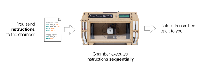
You can now send instructions to the chamber and receive data in real time. There are three types of [instructions](/the-chambers/how-they-work#chamber-control-language).

{% tabs %}
{% tab title="SET instruction" %}
{% code fullWidth="true" %}

```python
chamber.set(target, value)
```

{% endcode %}

This sets the variable `target` to the given `value`, returning when the change has been made in the hardware. The above call returns `None`.

See the [configuration docs](/the-chambers/how-they-work) for a list of variables and their valid / default values.
{% endtab %}

{% tab title="MEASURE instruction" %}

```python
data = chamber.measure(n, delay)
```

The chamber returns `n` successive measurements of all variables, including images if it produces them. Setting `delay` (in milliseconds) adds an additional delay between measurements, i.e., allowing you to change the measurement frequency.

If the chamber produces images, `data = (dataframe, images)` is a tuple of a pandas dataframe and an image array; otherwise it is just a pandas dataframe. See the [API Reference](broken://spaces/n3swfeDaIv3d3HxHu2q6) for more details.
{% endtab %}

{% tab title="WAIT instruction" %}

```python
chamber.wait(milliseconds)
```

The chamber acts as a precise clock and waits the given `milliseconds` before executing the next instruction.
{% endtab %}
{% endtabs %}
{% endstep %}
{% endstepper %}

{% hint style="info" %}
To ensure experimental consistency, the chamber accepts only one active connection at a time; starting a new connection will invalidate the previous one. For long-running experiments and multiple users, we recommend using the [experiment queue](/remote-lab/using-the-experiment-queue).
{% endhint %}

### A complete example

Let's connect to a [Light Tunnel Mk2](/the-chambers/light-tunnel-mk2) and collect images in real time.

```python
import causalchamber.lab as lab

# Open a real-time connection
chamber = lab.Chamber(chamber_id = 'lt-demo-ch4lu',
                      config = 'camera_fast',
                      credentials_file = '.credentials')

# Turn on the light source to red and take one image
chamber.set('red', 255)
df, images = chamber.measure(n=1)
```

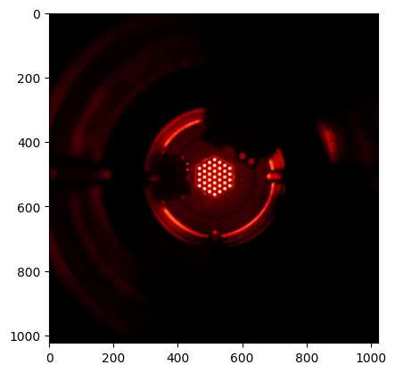
The returned data consists of two parts: `df` is a dataframe containing the sensor measurements, and `images` an array with the collected images (only one in this case).

Let's have a look at the resulting image.

```python
# Plot the image
import matplotlib.pyplot as plt
plt.imshow(images[0])
```

<div data-with-frame="true"><figure><img src="https://3492874807-files.gitbook.io/~/files/v0/b/gitbook-x-prod.appspot.com/o/spaces%2FUqYDL9yvLTNUYW7H1Q6t%2Fuploads%2FeBWEvJkbr2MDg8Ytcoer%2Fpackage_rt_sample_image.png?alt=media&amp;token=41f5e8d3-767b-4f10-b44b-c053705729a0" alt="" width="332"><figcaption></figcaption></figure></div>

### Submitting multiple instructions at once

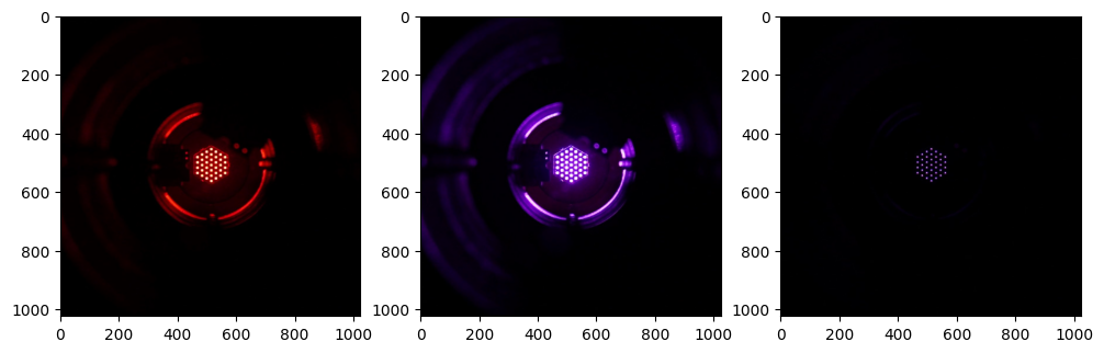
You can submit multiple instructions in a single batch. This saves you the round-trip to the chamber for each instruction and ensures consistent timing between instructions.

The data produced during the execution of the batch will be returned in `batch.submit()`.

```python
# Start a new batch
batch = chamber.new_batch()

# Add instructions
batch.set('red', 128)
batch.measure(n=1) # Image 1: red
batch.set('blue', 128)
batch.measure(n=1) # Image 2: purple
batch.set('pol_1', 90)
batch.measure(n=1) # Image 3: purple + crossed polarizers

# Submit the batch and receive the data
df, images = batch.submit()
```

To plot the resulting images:

<pre class="language-python"><code class="lang-python"><strong># Plot the images
</strong>plt.figure(figsize=(9,3))
for i,im in enumerate(images):
    plt.subplot(1,3,i+1)
    plt.imshow(im)
</code></pre>

<figure><img src="https://3492874807-files.gitbook.io/~/files/v0/b/gitbook-x-prod.appspot.com/o/spaces%2FUqYDL9yvLTNUYW7H1Q6t%2Fuploads%2Fjbc90DGB5gSnjijDfZyL%2Fpackage_rt_sample_images.png?alt=media&amp;token=cda6d748-380c-4322-91e7-200b234188b3" alt=""><figcaption></figcaption></figure>


# Using the experiment queue

We recommend using the queue for long-running experiments that require no interaction.

The queue works like a compute cluster: you submit an experiment protocol, the chamber runs it when ready, and it uploads the data to a server for you to download.

{% hint style="info" %}
We store your experimental data for the entire duration of your contract.
{% endhint %}

### Basic workflow

The API is very similar to that of the [real-time experiments](/remote-lab/running-a-real-time-experiment). You can find a [complete example](#a-complete-example) below.

{% stepper %}
{% step %}
**Connect to the Remote Lab**

First, open a connection to the remote lab (see also [Quickstart](/remote-lab/quickstart))

{% tabs %}
{% tab title="Credentials file" %}

```python
import causalchamber.lab as lab

rlab = lab.Lab(credentials_file = 'path/to/file')
```

{% endtab %}

{% tab title="Environment variables" %}
If you stored your credentials in environment variables, e.g., `USER` and `KEY`

```python
import os
import causalchamber.lab as lab

rlab = lab.Lab(credentials=(os.getenv('USER'), os.getenv('KEY')))
```

{% endtab %}
{% endtabs %}
{% endstep %}

{% step %}
**Create a new experiment protocol**

Then, start a new protocol by specifying which chamber (`chamber_id`) and [hardware configuration](/the-chambers/how-they-work) (`config`) you want it to run on

```python
experiment = rlab.new_experiment(chamber_id, config)
```

{% endstep %}

{% step %}
**Add instructions**

Add instructions to the experiment protocol

{% tabs %}
{% tab title="SET instruction" %}
{% code fullWidth="true" %}

```python
experiment.set(target, value)
```

{% endcode %}

This sets the variable `target` to the given `value`, returning when the change has been made in the hardware. The above call returns `None`.

See the [configuration docs](/the-chambers/how-they-work) for a list of variables and their valid / default values.
{% endtab %}

{% tab title="MEASURE instruction" %}

```python
experiment.measure(n, delay)
```

The chamber returns `n` successive measurements of all variables, including images if it produces them. Setting `delay` (in milliseconds) adds an additional delay between measurements, i.e., allowing you to change the measurement frequency.

If the chamber produces images, `data = (dataframe, images)` is a tuple of a pandas dataframe and an image array; otherwise it is just a pandas dataframe. See the [API Reference](broken://spaces/n3swfeDaIv3d3HxHu2q6) for more details.
{% endtab %}

{% tab title="WAIT instruction" %}

```python
experiment.wait(milliseconds)
```

The chamber acts as a precise clock and waits the given `milliseconds` before executing the next instruction.
{% endtab %}
{% endtabs %}

You can check which instructions are already in the protocol by calling `experiment.instructions`. Calling `experiment.clear()` will remove all instructions.

{% hint style="info" %}
You can also generate instructions directly [from a pandas dataframe](#generating-instructions-from-a-pandas-dataframe) (see below).
{% endhint %}
{% endstep %}

{% step %}
**Submit your experiment**

Once you are ready, submit the experiment to the chamber's queue with

```python
experiment.submit(tag='optional-tag')
```

This will return a `experiment_id` that uniquely identifies your experiment in the system.

To help you keep track of your experiments, you can also add an optional `tag` parameter with a string of your choice (alphanumeric characters and `+-_:`).
{% endstep %}
{% endstepper %}

### Monitoring your experiments

You can check on all your current and past experiments with

```python
rlab.get_experiments(print_max=10) # 0 for no print, None to print all
```

<mark style="color:$primary;">Output</mark>

<figure><img src="https://3492874807-files.gitbook.io/~/files/v0/b/gitbook-x-prod.appspot.com/o/spaces%2FUqYDL9yvLTNUYW7H1Q6t%2Fuploads%2FMF7oYTyGbtUuOAudDU73%2Fget_experiments.jpg?alt=media&amp;token=216c4a5c-a3cb-4457-87e1-3afac909998c" alt=""><figcaption></figcaption></figure>

You can also query the details (incl. status) for an individual experiment with

```python
rlab.get_experiment(experiment_id)
```

### Checking your position in the queue

You can monitor the running and queued experiments for a given chamber by calling

```python
rlab.get_queue(chamber_id)
```

<mark style="color:$primary;">Output</mark>

<figure><img src="https://3492874807-files.gitbook.io/~/files/v0/b/gitbook-x-prod.appspot.com/o/spaces%2FUqYDL9yvLTNUYW7H1Q6t%2Fuploads%2FI6LcK4INXqQsn2CEvEzF%2Fget_queue.jpg?alt=media&amp;token=2e2cd11e-db9a-4a54-b77e-0ca92537814f" alt=""><figcaption></figcaption></figure>

### Cancelling an experiment

You can cancel a <mark style="color:$warning;">`QUEUED`</mark> or <mark style="color:green;">`RUNNING`</mark> experiment by calling

```python
rlab.cancel_experiment(experiment_id)
```

For <mark style="color:green;">`RUNNING`</mark> experiments, the experiment will temporarily transition to status <mark style="color:purple;">`STOPPING`</mark> while the chamber finishes executing the current instruction. This may take a moment if that happens to be a long [measure](#measure-instruction) or [wait](#wait-instruction) instruction.

### Downloading the data

Once an experiment is finished (status=<mark style="color:$success;">`DONE`</mark>), you can download the data by calling

```python
data = rlab.download_data(experiment_id, root='path/to/download/dir')
```

where `root` specifies the directory where you want to store the data. Then, load the data into the desired format

```python
data.dataframe       # measurements as a pandas dataframe
data.image_arrays    # list of image arrays (H x W x 3)
data.image_iterator  # iterator over image arrays
```

### A complete example

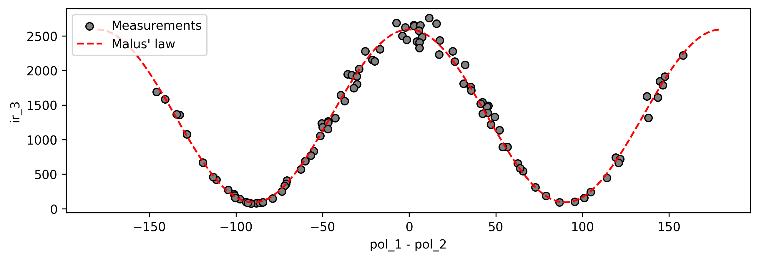
Let's submit an experiment to visualize the effect of [Malus' law of polarization](https://en.wikipedia.org/wiki/Polarizer#Malus's_law_and_other_properties) in the [Light Tunnel Mk2](/the-chambers/light-tunnel-mk2). You can learn more about this effect in [Appendix IV.2.1](https://arxiv.org/pdf/2404.11341#page=31.71) of the original chambers [paper](https://www.nature.com/articles/s42256-024-00964-x).

For our experiment, we will keep the light source fixed at a constant brightness and take measurements for random polarizer positions.

```python
import causalchamber.lab as lab
import numpy.random as random

# Connect to the remote lab
rlab = lab.Lab(credentials_file='.credentials')

# Start a new experiment protocol
experiment = rlab.new_experiment(chamber_id = 'lt-demo-ch4lu', config = 'standard')

# Add instructions
[experiment.set(color, 255) for color in ['red', 'green', 'blue']]
for i in range(100):
    # Set polarizers to random positions
    experiment.set('pol_1', random.uniform(-90,90))
    experiment.set('pol_2', random.uniform(-90,90))
    # Take one measurement
    experiment.measure(n=1)

# Submit the experiment
experiment_id = experiment.submit(tag='demo-malus')
```

You can monitor the experiment with `rlab.get_experiments()` and load the measurements into a pandas dataframe once it's done.

```python
data = rlab.download_data(experiment_id, root='/tmp')
df = data.dataframe
```

Now we can plot the light intensity after both polarizers vs. their relative angle (see `ir_3`, `pol_1`, `pol_2` in the [configuration docs](https://cchamber-box.s3.eu-central-2.amazonaws.com/config_doc_lt_mk2_standard.pdf)). For comparison, we show the prediction from [Malus' law](https://arxiv.org/pdf/2404.11341#page=31.71) in red.

```python
import matplotlib.pyplot as plt
import numpy as np

plt.figure(figsize=(8,3))

# Plot light intensity vs. relative polarizer angle
plt.scatter(df.pol_1 - df.pol_2, df.ir_3, c='gray', edgecolor='black')

# Plot Malus' law
x = np.arange(-180,180)
plt.plot(x, 92.30 + 2499.65 * np.cos(np.radians(x))**2, 'r--')

plt.legend(['Measurements', "Malus' law"], loc='upper left')
plt.xlabel('pol_1 - pol_2'); plt.ylabel('ir_3')
```

<figure><picture><source srcset="/files/bOnsdnwI1PnAz7OYdhty" media="(prefers-color-scheme: dark)"><img src="https://3492874807-files.gitbook.io/~/files/v0/b/gitbook-x-prod.appspot.com/o/spaces%2FUqYDL9yvLTNUYW7H1Q6t%2Fuploads%2FJjjkw4WYtvOtJZMXF5n0%2Fmalus_light.png?alt=media&amp;token=275835df-0ac2-4150-87f5-325f9aed1968" alt=""></picture><figcaption></figcaption></figure>

### Generating instructions from a pandas dataframe

To make things easier when creating experiments, you can also generate instructions from a pandas dataframe by calling [`experiment.from_df(...)`](broken://spaces/n3swfeDaIv3d3HxHu2q6) . For example, the above experiment can be rewritten as

```python
import causalchamber.lab as lab
import numpy.random as random
import pandas as pd

# Connect to the remote lab
rlab = lab.Lab(credentials_file='.credentials')

# Start a new experiment protocol
experiment = rlab.new_experiment(chamber_id = 'lt-demo-ch4lu', config = 'standard')

# Add instructions
[experiment.set(color, 255) for color in ['red', 'green', 'blue']]
df = pd.DataFrame({
    'pol_1': random.uniform(-90, 90, size=100),
    'pol_2': random.uniform(-90, 90, size=100)
})
experiment.from_df(df)

# Submit the experiment
experiment_id = experiment.submit(tag='demo-malus')
```

You can find more details about how the function works (e.g., to customize the number of measurements per row) in its [docstring](https://github.com/juangamella/causal-chamber-package/blob/1f1579ce4933c5a1ee3b5561f2a638aefc2ea215/causalchamber/lab/chamber.py#L590).


# Error handling & support

The causalchamber [package](https://github.com/juangamella/causal-chamber-package) can raise two types of errors

<table data-header-hidden><thead><tr><th width="145.614990234375">Error</th><th>Description</th></tr></thead><tbody><tr><td><code>LabError</code></td><td>This indicates an error on our side, e.g., due to a hardware failure or an internal server error.</td></tr><tr><td><code>UserError</code></td><td>These can arise during normal operation of the system—e.g., you reached the limit of queued experiments—or result from an error on your side, such as setting incorrect credentials or submitting an invalid instruction.</td></tr></tbody></table>

In either case, if an error persists or you are stuck, please let us know so we can help you. You can reach us at <support@causalchamber.ai> or through any of the support channels provided during onboarding.

{% hint style="info" %}
See [Troubleshooting](/support/troubleshooting) for a list of common issues and how to solve them.
{% endhint %}

### Example

Let's trigger a `UserError` by sending an invalid instruction to a chamber.

```python
import causalchamber.lab as lab

# Open a real-time connection
chamber = lab.Chamber(chamber_id = 'lt-demo-ch4lu',
                      config = 'standard',
                      credentials_file = '.credentials')

# Submit an invalid instruction (value out of range)
chamber.set('red', 999)
```

This raises the following exception

```python
---------------------------------------------------------------------------
UserError                                 Traceback (most recent call last)
[Trace details omitted]
UserError: (code 400) Line 1: Value 999 for variable 'red' is above maximum 255
  Trace codes
      (chamber: c687d22c-d07e-4aec-8ef1-0fd3ae40b188)
    (scheduler: cc512e6c-c11f-43d2-afdb-030b3bae9847)
```

Besides a description of the error and the traceback, the exception also provides **trace codes**, e.g., the uuid strings `c687d22c-d07e-4aec-8ef1-0fd3ae40b188` and `cc512e6c-c11f-43d2-afdb-030b3bae9847`. These allow us to track your request through our entire stack.

### Reporting errors

{% hint style="info" %}
The best way to report an error is to send us the complete error trace, including the traceback and **trace codes**.
{% endhint %}

You can report an error through <support@causalchamber.ai> or any of the support channels provided during onboarding.


# How they work

The [first chambers](/the-chambers/original-prototypes) were developed at the [Seminar for Statistics](https://math.ethz.ch/sfs) of ETH Zurich, initially conceived as testbeds for causal inference algorithms. They were presented in an [open-access paper](https://www.nature.com/articles/s42256-024-00964-x) in Nature Machine Intelligence, together with their open-source [blueprints](https://github.com/juangamella/causal-chamber/tree/main/hardware) and a collection of [public datasets](https://github.com/juangamella/causal-chamber).

Since then, we have improved and expanded the [original prototypes](/the-chambers/original-prototypes) into the new Mk2 models, which you can operate through our [Remote Lab](/remote-lab/quickstart).

{% columns %}
{% column %}

<figure><img src="https://3492874807-files.gitbook.io/~/files/v0/b/gitbook-x-prod.appspot.com/o/spaces%2FUqYDL9yvLTNUYW7H1Q6t%2Fuploads%2F5PDrqgk4mQsoOhqNs8tM%2Fwt_mk2_light_background_150dpi.png?alt=media&amp;token=14504755-5714-426a-8924-a353b5cd9c86" alt=""><figcaption></figcaption></figure>

{% content-ref url="/pages/Z8eYHzIcJtk5X0kfzXli" %}
[Wind Tunnel Mk2](/the-chambers/wind-tunnel-mk2)
{% endcontent-ref %}
{% endcolumn %}

{% column %}

<figure><img src="https://3492874807-files.gitbook.io/~/files/v0/b/gitbook-x-prod.appspot.com/o/spaces%2FUqYDL9yvLTNUYW7H1Q6t%2Fuploads%2FNB1EuTFi2dgKBNs8mclg%2Flt_light_backround.png?alt=media&amp;token=8376721f-3c81-4a76-a8b0-0b9179c0038b" alt=""><figcaption></figcaption></figure>

{% content-ref url="/pages/nfKs9660N39HBagy17gT" %}
[Light Tunnel Mk2](/the-chambers/light-tunnel-mk2)
{% endcontent-ref %}
{% endcolumn %}
{% endcolumns %}

### What is a Chamber?

A Chamber contains a physical system and allows algorithms to control and measure its variables without human supervision. It provides validation tasks with a ground truth for a variety of algorithms from ML, AI, statistics, and engineering.

Because the physical system is well understood, we can provide a ground truth for tasks in causal inference and anomaly detection. We have also built [mechanistic models](https://arxiv.org/pdf/2404.11341#page=28) and [simulators](https://github.com/juangamella/causal-chamber-package/tree/main/causalchamber/simulators) of the physical phenomena inside the Chambers, which are particularly useful for studying problems in Sim2Real, Simulation-Based Inference, Hybrid Learning, and related fields. See the [case studies](https://docs.causalchamber.ai/case-studies/) for examples.

### Hardware configurations

A Chamber can operate under several configurations, exposing different variables of the underlying physical system. It can also set control inputs as functions of other sensor measurements, allowing for feedback mechanisms and tunable causal effects.

{% hint style="info" %}
Configurations are specified at the beginning of an experiment and loaded automatically by the Chamber.
{% endhint %}

<details>

<summary>Light Tunnel Mk2: hardware configurations</summary>

See the [hardware configurations](/the-chambers/light-tunnel-mk2#hardware-configurations) for the [Light Tunnel Mk2](/the-chambers/light-tunnel-mk2)

</details>

<details>

<summary>Wind Tunnel Mk2: hardware configurations</summary>

See the [hardware configurations](/the-chambers/wind-tunnel-mk2#hardware-configurations) for the [Wind Tunnel Mk2](/the-chambers/wind-tunnel-mk2)

</details>

### Chamber control language

<figure><img src="https://3492874807-files.gitbook.io/~/files/v0/b/gitbook-x-prod.appspot.com/o/spaces%2FUqYDL9yvLTNUYW7H1Q6t%2Fuploads%2FErryXiTKjEr5q0CPUu9J%2Fbasic_operation.svg?alt=media&amp;token=5500b3db-f059-4365-b064-e4b2eb736f47" alt=""><figcaption></figcaption></figure>

The Chambers are controlled through a simple language with three instructions.

{% tabs %}
{% tab title="SET instruction" %}
{% code fullWidth="true" %}

```
set(target, value)
```

{% endcode %}

This sets the variable `target` to the given `value`, returning when the change has been made in the hardware.

See the [hardware configurations](#hardware-configurations) of each chamber for a list of variables and their valid and default values.
{% endtab %}

{% tab title="MEASURE instruction" %}
{% code overflow="wrap" %}

```
measure(n, delay)
```

{% endcode %}

The chamber returns `n` successive measurements of all variables, including images if it produces them. Setting `delay` (in milliseconds) adds a delay between measurements, allowing you to change the measurement frequency.

{% hint style="info" %}
The maximum measurement frequency, i.e., with `delay=0,` is approx. 12Hz for the [Wind Tunnel Mk2](/the-chambers/wind-tunnel-mk2) and 10Hz for the [Light Tunnel Mk2](/the-chambers/light-tunnel-mk2).
{% endhint %}
{% endtab %}

{% tab title="WAIT instruction" %}
{% code overflow="wrap" %}

```
wait(milliseconds)
```

{% endcode %}

The chamber acts as a precise clock and waits for the given `milliseconds` before executing the next instruction.
{% endtab %}
{% endtabs %}

Instructions can be sent synchronously (see [real-time experiments](/remote-lab/running-a-real-time-experiment)) or as an experiment protocol, which is placed on a [queue](/remote-lab/using-the-experiment-queue) and executed when a Chamber becomes available.

{% columns %}
{% column %}
{% content-ref url="/pages/eQKb9IRV2ljJzz3GaO9e" %}
[Running a real-time experiment](/remote-lab/running-a-real-time-experiment)
{% endcontent-ref %}
{% endcolumn %}

{% column %}
{% content-ref url="/pages/6ismfrBNj2HgguBeI1Yt" %}
[Using the experiment queue](/remote-lab/using-the-experiment-queue)
{% endcontent-ref %}
{% endcolumn %}
{% endcolumns %}


# Light Tunnel Mk2

Exhaustive documentation including variables, configurations and physical effects.

{% columns %}
{% column %}

<figure><img src="https://3492874807-files.gitbook.io/~/files/v0/b/gitbook-x-prod.appspot.com/o/spaces%2FUqYDL9yvLTNUYW7H1Q6t%2Fuploads%2FNB1EuTFi2dgKBNs8mclg%2Flt_light_backround.png?alt=media&amp;token=8376721f-3c81-4a76-a8b0-0b9179c0038b" alt=""><figcaption></figcaption></figure>
{% endcolumn %}

{% column %}
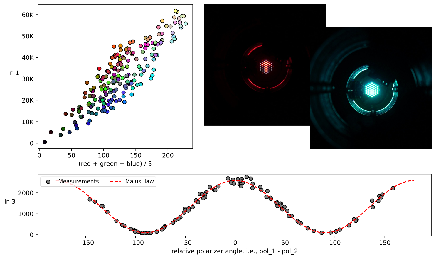
The Light Tunnel produces [**i.i.d.**](#user-content-fn-1)[^1] **data and images** from a controlled **optical experiment.**

It contains a controllable light source, linear polarizers mounted on rotating frames, and sensors to measure light intensity at different frequencies and locations. A camera captures images from inside the tunnel.
{% endcolumn %}
{% endcolumns %}

The chamber produces images and i.i.d. data from up to 99 [variables](#variables-table), including sensor measurements, control inputs, and sensor parameters.

<figure><picture><source srcset="/files/i9d1XaXEIWKgu9DpvXqr" media="(prefers-color-scheme: dark)"><img src="https://3492874807-files.gitbook.io/~/files/v0/b/gitbook-x-prod.appspot.com/o/spaces%2FUqYDL9yvLTNUYW7H1Q6t%2Fuploads%2Fb832TwJNi2O8XlQ4dj9N%2Flt-data-light-images.png?alt=media&amp;token=5a623acb-3b1a-4437-ad64-a5389b5d3052" alt="" width="563"></picture><figcaption><p><strong>Top right</strong>: infrared-intensity measurements produced by the first sensor (<code>ir_1</code>) for different intensities of the light-source channels (<code>red/green/blue</code>). <strong>Top left</strong>: examples of images produced by the tunnel in the linked_leds (left) and the camera_fast (right) <a href="#hardware-configurations">hardware configurations</a>. <strong>Bottom:</strong> observing Malus' law in the effect of the polarizer positions (<code>pol_1, pol_2</code>) on the infrared intensity at the third sensor (<code>ir_3</code>).</p></figcaption></figure>

<details>

<summary>Chamber diagram &#x26; variables</summary>

You can find a description of each variable in the documentation for each [hardware configuration](#hardware-configurations) below.

<figure><img src="https://3492874807-files.gitbook.io/~/files/v0/b/gitbook-x-prod.appspot.com/o/spaces%2FUqYDL9yvLTNUYW7H1Q6t%2Fuploads%2FKz8F7gs9Apgai4h7xHBc%2Flt_diagram_light_background.png?alt=media&amp;token=4a8cd377-6467-46df-b383-cefe553b7798" alt=""><figcaption><p>Right click to download the image (available under a <a href="https://creativecommons.org/licenses/by-nc/4.0/">CC BY-NC 4.0</a> non-commercial license).</p></figcaption></figure>

</details>

<details>

<summary>Simulators</summary>

See the [Simulator Index](https://github.com/juangamella/causal-chamber-package/tree/main/causalchamber/simulators) for a list of the simulators we offer for this chamber, including documentation and example code.

</details>

### Hardware configurations

Like all chambers, the wind tunnel can automatically load different [hardware configurations](/the-chambers/how-they-work#hardware-configurations). See the corresponding PDF for a chamber diagram, a complete description of all variables, and the causal ground-truth graph.

<table><thead><tr><th width="203.956787109375">Name</th><th width="77.6397705078125" data-type="checkbox">Img. data</th><th width="243.657958984375">Description</th><th width="149.1961669921875">Documentation</th><th>Causal ground-truth</th></tr></thead><tbody><tr><td><code>standard</code></td><td>false</td><td>Standard configuration with all variables (no camera) and exogenous inputs.</td><td><a href="https://cchamber-box.s3.eu-central-2.amazonaws.com/config_doc_lt_mk2_standard.pdf" class="button secondary">.pdf</a></td><td><a href="https://box.causalchamber.ai/gt_graph_lt_mk2_standard.pdf" class="button secondary">.pdf</a></td></tr><tr><td><code>linked_leds</code></td><td>false</td><td>Additional tunable causal effects.</td><td><a href="https://cchamber-box.s3.eu-central-2.amazonaws.com/config_doc_lt_mk2_linked_leds.pdf" class="button secondary">.pdf</a></td><td><a href="https://box.causalchamber.ai/gt_graph_lt_mk2_linked_leds.pdf" class="button secondary">.pdf</a></td></tr><tr><td><code>linked_leds_sigmoid</code></td><td>false</td><td>Same as <code>linked_leds</code> but with tunable non-linear effects.</td><td><a href="https://cchamber-box.s3.eu-central-2.amazonaws.com/config_doc_lt_mk2_linked_leds_sigmoid.pdf" class="button secondary">.pdf</a></td><td><a href="https://box.causalchamber.ai/gt_graph_lt_mk2_linked_leds.pdf" class="button secondary">.pdf</a></td></tr><tr><td><code>camera_fast</code></td><td>true</td><td>Provides images and camera variables.</td><td><a href="https://cchamber-box.s3.eu-central-2.amazonaws.com/config_doc_lt_mk2_camera_fast.pdf" class="button secondary">.pdf</a></td><td><a class="button secondary">.pdf</a></td></tr><tr><td><code>led_matrix</code></td><td>true</td><td>Same as <code>camera_fast</code> but with individual control of the light-source LEDs.</td><td><a href="https://cchamber-box.s3.eu-central-2.amazonaws.com/config_doc_lt_mk2_led_matrix.pdf" class="button secondary">.pdf</a></td><td><a class="button secondary">.pdf</a></td></tr></tbody></table>

### Map of effects

Here you can find a detailed description of all effects between chamber variables, together with additional experiments and figures. Throughout, we use an edge A $$\longrightarrow$$ B to denote that a variable A has an effect on variable B.

> **Short-hand notation**
>
> * A1/2 $$\longrightarrow$$ B, C is equivalent to the edges A1 $$\longrightarrow$$ B, A1 $$\longrightarrow$$ C, A2 $$\longrightarrow$$ B and A2 $$\longrightarrow$$ C
> * We can also express this as A\* $$\longrightarrow$$ B,C

Some text and figures in this section are adapted from the [original paper](https://www.nature.com/articles/s42256-024-00964-x) (Gamella et al. 2025, [Appendix III](https://static-content.springer.com/esm/art%3A10.1038%2Fs42256-024-00964-x/MediaObjects/42256_2024_964_MOESM1_ESM.pdf)).

{% hint style="info" %}
Some [hardware configurations](#hardware-configurations) introduce additional effects between variables. See their [documentation](#hardware-configurations) for the complete map of physical effects.
{% endhint %}

{% tabs %}
{% tab title="Graph" %}

<figure><img src="https://3492874807-files.gitbook.io/~/files/v0/b/gitbook-x-prod.appspot.com/o/spaces%2FUqYDL9yvLTNUYW7H1Q6t%2Fuploads%2F0dl0hAjgjprpflmkrUY3%2Flt_causal_graph_light.png?alt=media&amp;token=9cd94118-2374-4b9a-96fa-383d7eb4087e" alt=""><figcaption><p>Right click to download the image (available under a <a href="https://creativecommons.org/licenses/by-nc/4.0/">CC BY-NC 4.0</a> non-commercial license).</p></figcaption></figure>
{% endtab %}
{% endtabs %}

<details>

<summary>Causal ground-truth</summary>

The graph above can be interpreted as a **causal ground truth**, as formalized in Gamella et al. (2025, [Appendix V](https://cchamber-box.s3.eu-central-2.amazonaws.com/nature_paper_appendices.pdf)), i.e., an edge X $$\longrightarrow$$ Y signifies that—for some value of the other chamber inputs—an intervention on X will change the distribution of subsequent measurements of Y. The graph should <mark style="color:$danger;">**not**</mark> be taken as a graphical model of statistical dependencies, as [external influences](#external-influences) on the system may create additional correlations between variables. See the [research guide](/case-studies/causal-inference/generating-real-data-with-a-known-causal-structure#using-the-ground-truth-graph) for more details.

</details>

In what follows, we provide a detailed description and visualization of each edge (physical effect) in the above graph.

{% hint style="info" %}
See the [variables table](#variables-table) for a description of all variables in this section.
{% endhint %}

***

#### `red`, `green`, `blue` $$\longrightarrow$$ `ir_1/2/3`, `vis_1/2/3`

The brightness settings of the light-source colors (`red`, `green`, `blue`) affect the readings of the three light-intensity sensors. Each sensor produces two measurements: one for the infrared part of the spectrum (`ir_j`), and another for the visible part (`vis_j`). The effect of each color is approximately linear with heteroscedastic noise, and the slope is determined by its [typical wavelength](#user-content-fn-2)[^2] and the sensor's [spectral sensitivity](#user-content-fn-3)[^3].

{% tabs %}
{% tab title="Figure 1" %}

<figure><img src="https://3492874807-files.gitbook.io/~/files/v0/b/gitbook-x-prod.appspot.com/o/spaces%2FUqYDL9yvLTNUYW7H1Q6t%2Fuploads%2F0AupOSBrvZiN8N2fzeiG%2Frgb_on_sensors.svg?alt=media&amp;token=7347ed18-8a99-4cd1-b157-63a54c06dae4" alt=""><figcaption><p>Effect of each light-source color—controlled by the variables <code>red</code>, <code>green</code>, <code>blue</code>—on the measurements produced by the three light-intensity sensors <code>ir_1/2/3</code> and <code>vis_1/2/3</code>.  The sensors are placed at increasing distances from the light source (with the first sensor closest to it), resulting in a decrease in the maximum measurement value. The infrared channel (<code>ir_j</code>, top row) of the sensors is most sensitive to red light, whereas the effect is reversed for the visible channel (<code>vis_j</code>, bottom row).</p></figcaption></figure>
{% endtab %}

{% tab title="Experiment" %}
To recreate the data for the figure using the [Remote Lab](/remote-lab/quickstart):

{% code overflow="wrap" %}

```python
# Connect to the lab
import causalchamber.lab as lab
rlab = lab.Lab(credentials_file = '.credentials', verbose=False)

# Define experiment
experiment = rlab.new_experiment('lt-aeon-dlpv', 'standard')

rng = np.random.default_rng(42)

N = 300

colors = ['red', 'green', 'blue']

for i,value in zip(rng.choice([0,1,2], size=N), rng.integers(0,256,size=N)):
    # Set flag
    experiment.set('flag', i)
    # Set all colors to zero
    [experiment.set(cc, 0) for cc in colors]
    # Set random color value and take a measurement
    experiment.set(colors[i], value)
    experiment.measure(n=1)

# Submit
eid = experiment.submit(tag='ls-colors')
```

{% endcode %}
{% endtab %}
{% endtabs %}

#### `red`, `green`, `blue` $$\longrightarrow$$ `current_ls`, `current_ls_raw`

The chamber produces calibrated measurements (`current_ls`, in Amperes) of the electrical current drawn by the light source. For each measurement, the chamber also returns the underlying raw, uncalibrated measurement (`current_ls_raw`), which takes values in the range \[-2¹⁵, 2¹⁵] (the output of the sensor's [ADC](https://en.wikipedia.org/wiki/Analog-to-digital_converter)).

The effect of the brightness settings `red/green/blue` is approximately linear with the same slope for each color ([Figure 2](#figure-2)).

{% tabs %}
{% tab title="Figure 2" %}

<figure><img src="https://3492874807-files.gitbook.io/~/files/v0/b/gitbook-x-prod.appspot.com/o/spaces%2FUqYDL9yvLTNUYW7H1Q6t%2Fuploads%2Fuiu8i8YvOdwlKLoPQ5Ed%2Frgb_on_current.svg?alt=media&amp;token=fad9c292-8e40-4739-a8de-89eb0e099621" alt="" width="509"><figcaption><p>Measurements of the current drawn by the light source (<code>current_ls</code>) and the corresponding raw uncalibrated measurement (<code>current_ls_raw</code>), for different values of each color channel.</p></figcaption></figure>
{% endtab %}

{% tab title="Experiment" %}
To recreate the data for the figure using the [Remote Lab](/remote-lab/quickstart):

{% code overflow="wrap" %}

```python
# Connect to the lab
import causalchamber.lab as lab
rlab = lab.Lab(credentials_file = '.credentials', verbose=False)

# Define experiment
experiment = rlab.new_experiment('lt-aeon-dlpv', 'standard')

rng = np.random.default_rng(42)

N = 300

colors = ['red', 'green', 'blue']

for i,value in zip(rng.choice([0,1,2], size=N), rng.integers(0,256,size=N)):
    # Set flag
    experiment.set('flag', i)
    # Set all colors to zero
    [experiment.set(cc, 0) for cc in colors]
    # Set random color value and take a measurement
    experiment.set(colors[i], value)
    experiment.measure(n=1)

# Submit
eid = experiment.submit(tag='ls-colors')
```

{% endcode %}
{% endtab %}
{% endtabs %}

#### `offset/sps/res_current_ls` $$\longrightarrow$$`current_ls`, `current_ls_raw`

We can independently control three parameters of the analog sensor that produces the measurements `current_ls` and `current_ls_raw`:

* `offset_current_ls` : the reference voltage. Changing it creates an additive shift in the uncalibrated measurements (`current_ls_raw`) but is largely compensated for in the calibrated measurements ([Figure 3](#figure-3), left).
* `sps_current_ls` : the [oversampling rate](https://www.microchip.com/en-us/about/media-center/blog/2024/what-is-oversampling), i.e., how many readings are averaged to produce a single measurement. Lower values correspond to higher oversampling rates, increasing the noise-to-signal ratio of the resulting measurements. Both the calibrated and uncalibrated measurements are affected ([Figure 3](#figure-3), center).
* `res_current_ls` : the measurement range—and thus the resolution—of the sensor. Higher values correspond to smaller measurement ranges, increasing the resolution but saturating the sensor if the actual values fall outside this range ([Figure 3](#figure-3), right). Changes to `res_current_ls` result in a shift and scaling of the uncalibrated measurements (`current_ls_raw`).

{% tabs %}
{% tab title="Figure 3" %}

<figure><img src="https://3492874807-files.gitbook.io/~/files/v0/b/gitbook-x-prod.appspot.com/o/spaces%2FUqYDL9yvLTNUYW7H1Q6t%2Fuploads%2FlWB3eBWvILYH8V2AdfwP%2Foffset_sps_res_current_ls.svg?alt=media&amp;token=2e79e390-0049-42ee-a7f5-038c1fec03af" alt=""><figcaption><p>Effect of the sensor parameters <code>offset/sps/res_current_ls</code> (resp. left, center, right) on the calibrated (<code>current_ls</code>, top) and uncalibrated (<code>current_ls_raw</code>, bottom) measurements of the current drawn by the light source. The left and center plot show measurements for <code>red=green=blue=0</code>, and the right plot shows measurements for <code>red=green=blue</code> sampled from random values in <code>[0,255]</code>. The calibrated measurements (in Amps) largely compensate for changes in the reference voltage (<code>offset_current_ls</code>, left top) and sensor resolution (<code>res_current_ls</code>, right top), unless sensor saturation occurs. For example, in the right plot, at resolution <code>res_current_ls = 2</code>, the measurements fall outside of the sensor range, resulting in a saturation of the sensor output. Both calibrated and uncalibrated measurements are affected by changes in the oversampling rate (<code>sps_current_ls</code>, center) which affects their signal-to-noise ratio (i.e., variance, precision).</p></figcaption></figure>
{% endtab %}

{% tab title="Experiment" %}
You can replicate the experiments for this plot with the [Remote Lab](/remote-lab/quickstart). For the left panel (varying `offset_current_ls`):

{% code overflow="wrap" %}

```python
# Connect to the lab
import causalchamber.lab as lab
rlab = lab.Lab(credentials_file = '.credentials', verbose=False)

# Declare experiment
experiment = rlab.new_experiment(chamber_id = 'lt-aeon-dlpv', config='standard')

# Iterate over offset values and take measurements
for offset in [0, 100, 200, 300]:
    experiment.set('offset_current_ls', offset)
    experiment.measure(n=500)

# Submit
experiment.submit(tag='offset-current-ls')
```

{% endcode %}

For the center panel (varying `sps_current_ls`):

{% code overflow="wrap" %}

```python
# Connect to the lab
import causalchamber.lab as lab
rlab = lab.Lab(credentials_file = '.credentials', verbose=False)

# Declare experiment
experiment = rlab.new_experiment(chamber_id = 'lt-aeon-dlpv', config='standard')

# Iterate over sps values and take measurements
for sps in [0, 2, 5, 7]:
    experiment.set('sps_current_ls', sps)
    experiment.measure(n=100)

# Submit
experiment.submit(tag='sps-current-ls')
```

{% endcode %}

For the right panel (varying `res_current_ls`):

{% code overflow="wrap" %}

```python
import numpy.random as np
import pandas as pd

# Connect to the lab
import causalchamber.lab as lab
rlab = lab.Lab(credentials_file = '.credentials', verbose=False)

# Declare experiment
experiment = rlab.new_experiment(chamber_id = 'lt-aeon-dlpv', config='standard')

# Iterate over res values and take measurements for different light source brightness
for res in np.arange(3):
    experiment.set('res_current_ls', res)    
    experiment.from_df(
        pd.DataFrame({c: np.arange(256) for c in ['red', 'green', 'blue']})                      
    )

# Submit
experiment.submit(tag='res-current-ls')
```

{% endcode %}
{% endtab %}
{% endtabs %}

#### `diode_ir_j` $$\longrightarrow$$ `ir_j`, `diode_vis_j` $$\longrightarrow$$ `vis_j` (j = 1, 2, 3)

We can control the size of the photodiode used by each sensor to produce the light-intensity measurements `ir_j` and `vis_j`. There are three photodiodes (`diode_ir_j=0,1,2`) for the infrared channel (`ir_j`) and two photodiodes (`diode_vis_j=0,1`) for the visible channel (`vis_j`). Larger values correspond to larger photodiodes, which collect light over a greater area, increasing the sensor's sensitivity.

{% tabs %}
{% tab title="Figure 4" %}

<figure><img src="https://3492874807-files.gitbook.io/~/files/v0/b/gitbook-x-prod.appspot.com/o/spaces%2FUqYDL9yvLTNUYW7H1Q6t%2Fuploads%2FPlHdQ2FlFOZ5DS6PHm4z%2Fdiodes.svg?alt=media&amp;token=ee6ee899-a912-4b8c-b114-5a54afd4459d" alt=""><figcaption><p>Measurements from the three light sensors (left / center / right) and their two channels (infrared, top; visible, bottom), for different photodiode settings, under random brightness settings of the light source's <code>green</code> channel. Increasing the diode size—i.e., larger values of <code>diode_ir/vis_j</code>—increases the sensitivity of the sensor.</p></figcaption></figure>
{% endtab %}

{% tab title="Experiment" %}
To recreate the data for the figure using the [Remote Lab](/remote-lab/quickstart):

{% code overflow="wrap" %}

```python
# Connect to the lab
import causalchamber.lab as lab
import numpy.random as random

rlab = lab.Lab(credentials_file = '.credentials', verbose=False)

# Declare experiment
experiment = rlab.new_experiment(chamber_id = 'lt-aeon-dlpv', config='standard')

# Inputs: random green color and diode sizes
N = 1000
inputs = pd.DataFrame({'green': random.randint(0,256,size=N),
                       'diode_ir_1': random.choice([0,1,2], size=N),
                       'diode_ir_2': random.choice([0,1,2], size=N),
                       'diode_ir_3': random.choice([0,1,2], size=N),
                       'diode_vis_1': random.choice([0,1], size=N),
                       'diode_vis_2': random.choice([0,1], size=N),
                       'diode_vis_3': random.choice([0,1], size=N)})

# One measurement per combination
experiment.from_df(inputs)

# Submit
experiment.submit(tag='diodes')
```

{% endcode %}
{% endtab %}
{% endtabs %}

#### `t_ir_j` $$\longrightarrow$$ `ir_j`, `t_vis_j` $$\longrightarrow$$ `vis_j` (j = 1, 2, 3)

We can also control the exposure time of each light sensor, affecting its sensitivity. Changes to the exposure time (i.e., [integration time](https://en.wikipedia.org/wiki/Integrating_ADC)) also affect the properties of the sensor noise, changing the conditional distribution of the measurements given the light source brightness (see XY in Figure Y below). A timing mechanism ensures that changes in the exposure time do not affect the overall measurement time.

{% tabs %}
{% tab title="Figure 5" %}

<figure><img src="https://3492874807-files.gitbook.io/~/files/v0/b/gitbook-x-prod.appspot.com/o/spaces%2FUqYDL9yvLTNUYW7H1Q6t%2Fuploads%2FtJf0P1EItQk10OamEWkK%2Fintegration_times.svg?alt=media&amp;token=bc1f42bd-9171-436a-8d08-85ec151eba32" alt=""><figcaption><p>Measurements from the three light sensors (left / center / right) and their two channels (infrared, top; visible, bottom), for different exposure settings, under random brightness settings of the light source's <code>green</code> channel. Increasing the exposure time—i.e., <a href="https://en.wikipedia.org/wiki/Integrating_ADC">integration time</a>—increases the sensitivity of the sensor and affects the noise distribution; see, e.g., the difference between <code>t_ir/vis_j=3</code> and <code>t_ir/vis_j=2</code> above.</p></figcaption></figure>
{% endtab %}

{% tab title="Experiment" %}
To recreate the data for the figure using the [Remote Lab](/remote-lab/quickstart):

{% code overflow="wrap" %}

```python
# Connect to the lab
import causalchamber.lab as lab
import numpy.random as random

rlab = lab.Lab(credentials_file = '.credentials', verbose=False)

# Declare experiment
experiment = rlab.new_experiment(chamber_id = 'lt-aeon-dlpv', config='standard')

# Inputs: random green color and exposure times (t_*)
N = 1000
inputs = pd.DataFrame({'green': random.randint(0,256,size=N),
                       't_ir_1': random.choice([0,1,2,3], size=N),
                       't_ir_2': random.choice([0,1,2,3], size=N),
                       't_ir_3': random.choice([0,1,2,3], size=N),
                       't_vis_1': random.choice([0,1,2,3], size=N),
                       't_vis_2': random.choice([0,1,2,3], size=N),
                       't_vis_3': random.choice([0,1,2,3], size=N)})

# One measurement per combination
experiment.from_df(inputs)

# Submit
experiment.submit(tag='exposure')
```

{% endcode %}
{% endtab %}
{% endtabs %}

#### `pol_j` $$\longrightarrow$$ `angle_j`, `angle_j_raw`, `angle_j_digital` (j = 1, 2)

The position settings `pol_1/2` determine the position (in degrees) of the two polarizer frames. The actual position is measured by two sensors: an encoder producing the measurements `angle_1/2_digital` , and an analog sensor producing `angle_1/2`, both in degrees. For the latter, the chamber also returns the underlying raw, uncalibrated measurements (`angle_1/2_raw`), which take values in the range \[-2¹⁵, 2¹⁵] (the output of the sensor's [ADC](https://en.wikipedia.org/wiki/Analog-to-digital_converter)). The relationship between the position setting and the angle measurements is modulated by the motor parameters (see below) and the [parameters](#offset-res-sps_angle_j-angle_j-angle_j_raw-j-1-2) of the analog sensor.

{% tabs %}
{% tab title="Figure 6" %}

<figure><img src="https://3492874807-files.gitbook.io/~/files/v0/b/gitbook-x-prod.appspot.com/o/spaces%2FUqYDL9yvLTNUYW7H1Q6t%2Fuploads%2FpJlXjzJBEgRCRLfndf8y%2Fpolarizers_angle1.svg?alt=media&amp;token=8c39b43c-f961-4cef-ae34-200b4cde95df" alt=""><figcaption><p>Angle measurements <code>angle_1_digital</code> (left, in degrees), <code>angle_1</code> (center, in degrees) and <code>angle_1_raw</code> (right) for 1000 polarizer positions <code>pol_1</code> sampled uniformly at random from the range <code>[-90,90]</code> . The behaviour for the second polarizer (i.e., <code>pol_2</code>, <code>angle_2_*</code>) is the same and not shown.</p></figcaption></figure>
{% endtab %}

{% tab title="Experiment" %}
To recreate the data for the figure using the [Remote Lab](/remote-lab/quickstart):

{% code overflow="wrap" %}

```python
import numpy.random as rand
import pandas as pd

# Connect to the lab
import causalchamber.lab as lab
rlab = lab.Lab(credentials_file = '.credentials', verbose=False)

# Declare experiment
experiment = rlab.new_experiment(chamber_id = 'lt-aeon-dlpv', config='standard')

# Take measurements at random polarizer positions
experiment.from_df(
    pd.DataFrame({'pol_1': rand.uniform(-90,90,1000)})
)

# Submit
experiment.submit(tag='pol-random')
```

{% endcode %}
{% endtab %}
{% endtabs %}

**Motor parameters**

The relationship between the position settings `pol_1/2` and the actual polarizer positions—as measured by angle\_1/2, angle\_1/2\_raw, and angle\_1/2\_digital—is further modulated by the motor parameters.

For example, lowering the resolution of the motor (`mot_1/2_steps`) results in a coarser polarizer placement. If we lower the current delivered to the motors (`mot_1/2_max`) or power them off completely (`mot_1/2_enabled = 0`), they will cease to function properly, missing steps and creating a mismatch between `pol_1/2` and the actual positions measured by `angle_*` ([Figure 7](#figure-7)).

{% tabs %}
{% tab title="Figure 7" %}

<figure><img src="https://3492874807-files.gitbook.io/~/files/v0/b/gitbook-x-prod.appspot.com/o/spaces%2FUqYDL9yvLTNUYW7H1Q6t%2Fuploads%2FAMxoEngMUaV0SmgDlj73%2Fmotor_parameters.svg?alt=media&amp;token=9a4bd788-291d-4a1b-b4ea-213a845175c1" alt=""><figcaption><p>Position of the first polarizer (<code>angle_1</code>) along a trajectory (dotted black line) defined by the input <code>pol_1</code> that sets the desired polarizer position. We show trajectories for the default motor parameters (left) and different values of the motor parameters <code>mot_1_max/enabled</code>. Lowering the current delivered to the motor (<code>mot_1_max</code>), or powering it off completely (<code>mot_1_enabled = 0</code>) cause the motor to miss steps, creating a mismatch between the set position (<code>pol_1</code>) and the actual position of the hatch (<code>angle_1</code>). The behavior for the second polarizer (<code>pol_2</code>, <code>angle_2</code>) and the digital angle measurements (<code>angle_1/2_digital</code>) is the same and not shown.</p></figcaption></figure>
{% endtab %}

{% tab title="Experiment" %}
To recreate the data for the figure using the [Remote Lab](/remote-lab/quickstart):

{% code overflow="wrap" %}

```python
# Connect to the lab
import causalchamber.lab as lab
rlab = lab.Lab(credentials_file = '.credentials', verbose=False)

# Experiment setup
i = 1 # polarizer number
ids = {}
settings = [None, # default settings
            {f'mot_{i}_max': 1024},
            {f'mot_{i}_max': 512},
            {f'mot_{i}_max': 256},
            {f'mot_{i}_enabled': 0},            
           ]

# Run a separate experiment for each setting
for setting in settings:    
    experiment = rlab.new_experiment(chamber_id = 'lt-aeon-dlpv', config='standard')

    # Set experiment settings
    if setting is None:
        label = "default"
    else:
        label = "-".join([f'{p}:{v}' for p,v in setting.items()])
        for var,value in setting.items():
            experiment.set(var, value)
    
    # Trajectory for the polarizer
    if "steps" in label:
        t =  4 * np.cos(np.linspace(0, 2*np.pi, 25)) - 8
    else:
        t =  90 * np.cos(np.linspace(0, 2*np.pi, 25)) - 90
    for pol in (t):
        experiment.set(f'pol_{i}', pol)
        experiment.measure(n=1)
    
    # Submit    
    # experiment.submit(tag=label)
    ids[label.replace(":", "=").replace("-", ", ")] = experiment.submit(tag=label)
```

{% endcode %}
{% endtab %}
{% endtabs %}

#### `mot_j_max/enabled` $$\longrightarrow$$ `current_mot_j`, `current_mot_j_raw` (j = 1, 2)

The variables `mot_1/2_max` control the amount of electrical current delivered to the each polarizer motor, and `mot_1/2_enabled` switch the motors on or off. Thus, they affect the calibrated (`current_mot_1/2`) and uncalibrated (`current_mot_1/2_raw`) measurements of the electrical current drawn by the polarizer motors. The effect of `mot_1/2_max` and `mot_1/2_enabled` on the current measurements is instantaneous, i.e., faster than the measurement rate ([Figure 8](#figure-8), left). The relationship between `mot_1/2_max` and `current_1/2_mot`, `current_mot_1/2_raw` is non-linear ([Figure 8](#figure-8), right).

{% tabs %}
{% tab title="Figure 8" %}

<figure><img src="https://3492874807-files.gitbook.io/~/files/v0/b/gitbook-x-prod.appspot.com/o/spaces%2FUqYDL9yvLTNUYW7H1Q6t%2Fuploads%2FODLqr3SUTMEJHNzowc8f%2Fmot_1_max.svg?alt=media&amp;token=2e980d2a-35f7-4b36-95df-d98a53585aeb" alt=""><figcaption><p><strong>Left:</strong> calibrated motor current (<code>current_mot_1</code>) under an impulse on the input <code>mot_1_max</code> , when the motor is enabled (<code>mot_1_enabled=1</code>, blue) and when it is disabled (<code>mot_1_enabled=0</code>, yellow). <strong>Right:</strong> measurements of the calibrated motor current (<code>current_mot_1</code>) for different values of <code>mot_1_max</code>, when the motor is enabled (<code>mot_1_enabled=1</code>, blue) and when it is disabled (<code>mot_1_enabled=0</code>, yellow). The behavior of the second motor and the uncalibrated measurements <code>current_mot_1/2_raw</code> is the same and not shown.</p></figcaption></figure>
{% endtab %}

{% tab title="Experiment" %}
To replicate the experiment for the left panel (impulse) using the [Remote Lab](/remote-lab/quickstart):

{% code overflow="wrap" %}

```python
# Connect to the lab
import causalchamber.lab as lab
rlab = lab.Lab(credentials_file = '.credentials', verbose=False)

# Declare experiment
experiment = rlab.new_experiment(chamber_id = 'lt-aeon-dlpv', config='standard')

# Toggle motor on and off
pol = 1
for enabled in [0,1]:
    experiment.set(f'mot_{pol}_enabled', enabled)
    #   Apply impulse
    experiment.set(f'mot_{pol}_max', 0)
    experiment.measure(20)
    experiment.set(f'mot_{pol}_max', 4095)
    experiment.measure(30)
    experiment.set(f'mot_{pol}_max', 0)
    experiment.measure(50)

# Submit
experiment.submit(tag='mot-max-impulse')
```

{% endcode %}

For the right panel:

{% code overflow="wrap" %}

```python
# Connect to the lab
import causalchamber.lab as lab
rlab = lab.Lab(credentials_file = '.credentials', verbose=False)

# Declare experiment
experiment = rlab.new_experiment(chamber_id = 'lt-aeon-dlpv', config='standard')

# Set motor current at random
rng = np.random.default_rng(134)
pol = 1
for enabled in [0,1]:
    experiment.set(f'mot_{pol}_enabled', enabled)
    for i in range(1000):
        experiment.set(f'mot_{pol}_max', rng.choice(np.arange(4096)))
        experiment.measure(n=1)

# Submit
experiment.submit(tag='mot-max-random')
```

{% endcode %}
{% endtab %}
{% endtabs %}

#### `offset/res/sps_angle_j` $$\longrightarrow$$ `angle_j`, `angle_j_raw` (j = 1, 2)

We can independently control three parameters of the analog sensors that produce the measurements `angle_1/2` and `angle_1/2_raw`:

* `offset_angle_1/2` : the reference voltage. Changing it creates an additive shift in the uncalibrated measurements (`angle_1/2_raw`) but is largely compensated for in the calibrated measurements ([Figure 9](#figure-9), left).
* `sps_angle_1/2` : the [oversampling rate](https://www.microchip.com/en-us/about/media-center/blog/2024/what-is-oversampling), i.e., how many readings are averaged to produce a single measurement. Lower values correspond to higher oversampling rates, increasing the noise-to-signal ratio of the resulting measurements. Both the calibrated and uncalibrated measurements are affected ([Figure 9](#figure-9), center).
* `res_angle_1/2` : the measurement range—and thus the resolution—of the sensor. Higher values correspond to smaller measurement ranges, increasing the resolution but saturating the sensor if the actual values fall outside this range ([Figure 9](#figure-9), right). Changes to `res_angle_1/2` result in a shift and scaling of the uncalibrated measurements (`angle_1/2_raw`).

{% tabs %}
{% tab title="Figure 9" %}

<figure><img src="https://3492874807-files.gitbook.io/~/files/v0/b/gitbook-x-prod.appspot.com/o/spaces%2FUqYDL9yvLTNUYW7H1Q6t%2Fuploads%2FWi1boyx2oW2GpVeRQIXo%2Foffset_sps_res_angle_1.svg?alt=media&amp;token=d581e4c6-a594-49bb-a8ee-39c50906eff3" alt=""><figcaption><p>Effect of the sensor parameters <code>offset/sps/res_angle_1</code> (resp. left, center, right) on the calibrated (<code>angle_1</code>, top) and uncalibrated (<code>angle_1_raw</code>, bottom) measurements of the polarizer position. The behavior for the second polarizer is the same and not shown. The left and center plot show measurements for <code>pol_1=0</code>, and the right plot shows measurements for <code>pol_1</code> sampled from random values in <code>[-180,0]</code>. The calibrated measurements (in degrees) largely compensate for changes in the reference voltage (<code>offset_angle_1</code>, left top) and sensor resolution (<code>res_angle_1</code>, right top), unless sensor saturation occurs. For example, in the right plot, at resolution <code>res_angle_1 = 2</code>, the measurements fall outside of the sensor range, resulting in a saturation of the sensor output. Both calibrated and uncalibrated measurements are affected by changes in the oversampling rate (<code>sps_angle_1</code>, center), which affects their signal-to-noise ratio (i.e., variance, precision).</p></figcaption></figure>
{% endtab %}

{% tab title="Experiment" %}
You can replicate the experiments for this plot with the [Remote Lab](/remote-lab/quickstart). For the left panel (varying `offset_angle_1`):

{% code overflow="wrap" %}

```python
# Connect to the lab
import causalchamber.lab as lab
rlab = lab.Lab(credentials_file = '.credentials', verbose=False)

# Declare experiment
experiment = rlab.new_experiment(chamber_id = 'lt-aeon-dlpv', config='standard')

# Iterate over offset values and take measurements
for offset in [0, 100, 200, 300]:
    experiment.set('offset_angle_1', offset)
    experiment.measure(n=500)

# Submit
experiment.submit(tag='offset-current-led')
```

{% endcode %}

For the center panel (varying `sps_angle_1`):

{% code overflow="wrap" %}

```python
# Connect to the lab
import causalchamber.lab as lab
rlab = lab.Lab(credentials_file = '.credentials', verbose=False)

# Declare experiment
experiment = rlab.new_experiment(chamber_id = 'lt-aeon-dlpv', config='standard')

# Iterate over sps values and take measurements
for sps in [0, 2, 5, 7]:
    experiment.set('sps_angle_1', sps)
    experiment.measure(n=100)

# Submit
experiment.submit(tag='sps-current-led')
```

{% endcode %}

For the right panel (varying `res_angle_1`):

{% code overflow="wrap" %}

```python
import numpy.random as rand
import pandas as pd

# Connect to the lab
import causalchamber.lab as lab
rlab = lab.Lab(credentials_file = '.credentials', verbose=False)

# Declare experiment
experiment = rlab.new_experiment(chamber_id = 'lt-aeon-dlpv', config='standard')

# Iterate over res values and take measurements for different polarizer positions
for res in np.arange(3):
    experiment.set('res_angle_1', res)    
    experiment.from_df(
        pd.DataFrame({'pol_1': rand.uniform(-180, 0, size=200)})
    )

# Submit
experiment.submit(tag='res-current-angle-1')
```

{% endcode %}
{% endtab %}
{% endtabs %}

#### `pol_1/2` $$\longrightarrow$$ `ir_3`, `vis_3`

The position of the polarizers affects the intensity of the light passing through them, affecting the readings (`ir_3`, `vis_3`) of the third light sensor. The effect is described by Malus' law, i.e., the intensity $$I$$ after the polarizer pair is given by

$$
I = I\_0 \cos^2(\theta\_1 - \theta\_2),
$$

where $$I\_0$$ is the intensity before the polarizers, and $$\theta\_1, \theta\_2$$ are the polarizer positions. The above law holds for ideal polarizers; in practice, the polarizers do not block all light, and the resulting intensity is better approximated by

$$
I = I\_0\left\[T\_p - T\_c) \cos^2(\theta\_1 - \theta\_2) + T\_c\right],
$$

where $$T\_p, T\_c$$ are the polarizer's parallel and crossed transmission rates; see Gamella et al. (2025a, [Appendix IV.2.1](https://cchamber-box.s3.eu-central-2.amazonaws.com/nature_paper_appendices.pdf#page=18)) for more details. Note that transmission rates vary with wavelength; i.e., the polarizer blocks red light more than green or blue light, thereby changing the color of the captured images (see, e.g., Gamella et al. 2025b, [Figure 2CD](https://arxiv.org/pdf/2502.20099#page=3)).

{% tabs %}
{% tab title="Figure 10" %}

<figure><img src="https://3492874807-files.gitbook.io/~/files/v0/b/gitbook-x-prod.appspot.com/o/spaces%2FUqYDL9yvLTNUYW7H1Q6t%2Fuploads%2F8eJcYM3puWY9NjA6U3LN%2Fpolarizers.svg?alt=media&amp;token=4cdb33bf-4c0a-4007-8419-c40e9e78c46c" alt="" width="563"><figcaption><p>Effect of the polarizer positions <code>pol_1</code> and <code>pol_2</code> on the infrared (<code>ir_3</code>) and visible (<code>vis_3</code>) light-intensity measurements produced by the third sensor, which is placed behind both polarizers relative to the light source (see <a href="#chamber-diagram-and-variables">diagram</a>). In the experiment above, the polarizer positions are sampled uniformly at random while the light source is kept at a fixed brightness (for each of the <code>red</code>, <code>green</code> and <code>blue</code> channels).</p></figcaption></figure>
{% endtab %}

{% tab title="Experiment" %}
To recreate the data for the figure using the [Remote Lab](/remote-lab/quickstart):

{% code overflow="wrap" %}

```python

import causalchamber.lab as lab
import numpy.random as random
import pandas as pd

# Connect to the remote lab
rlab = lab.Lab(credentials_file='.credentials', verbose=False))

# Start a new experiment protocol
experiment = rlab.new_experiment(chamber_id = 'lt-aeon-dlpv', config = 'standard')

# Polarizer inputs
N = 300

# Repeat experiment for different colors
colors = ['red', 'green', 'blue']

for i, color in enumerate(colors):
    # Set flag
    experiment.set('flag', i)
    # Set all colors to zero
    [experiment.set(cc, 0) for cc in colors]
    # Set color channel to max
    experiment.set(color, 255)
    # Add polarizer inputs
    experiment.from_df(
        pd.DataFrame({
            'pol_1': random.uniform(-90, 90, size=N),
            'pol_2': random.uniform(-90, 90, size=N)
        }))

# Submit the experiment
experiment_id = experiment.submit(tag='polarizers')
```

{% endcode %}
{% endtab %}
{% endtabs %}

#### `led_j_ir`, `led_j_uv` $$\longrightarrow$$ `ir_j`, `vis_j` (j = 1, 2, 3)

Besides the light source, two additional LEDs placed by each light sensor have an effect on its readings. To avoid affecting the measurements of the other light sensors, the LEDs only turn on when their corresponding sensor is taking a measurement. There is an IR LED and a UV LED, with the settings `led_j_ir`, `led_j_uv` controlling the current flowing through them, and thus, their brightness. The IR LED can saturate the infrared measurements (`ir_1/2/3`) produced by the sensors ([Figure 11](#figure-11), top). TODO: experiment code

{% tabs %}
{% tab title="Figure 11" %}

<figure><img src="https://3492874807-files.gitbook.io/~/files/v0/b/gitbook-x-prod.appspot.com/o/spaces%2FUqYDL9yvLTNUYW7H1Q6t%2Fuploads%2FlxwEkZLDeVmZFt6abs9b%2Fleds_on_sensors.svg?alt=media&amp;token=2d3fa5cf-c654-4b8a-932a-4edafb8391a5" alt=""><figcaption><p>Effect of the by-sensor LEDs on the measurements of the three light sensors (left/center/right) and their infrared (<code>ir_1/2/3</code>, top) and visible (<code>vis_1/2/3</code>, bottom) channels. The LEDs turn on only when their corresponding sensor is taking a measurement and do not affect the measurements of the other sensors. The IR LED (<code>led_1/2/3_ir</code>) can cause the infrared measurements (<code>ir_1/2/3</code>) to saturate.</p></figcaption></figure>
{% endtab %}

{% tab title="Experiment" %}
To recreate the data for the figure using the [Remote Lab](/remote-lab/quickstart):

{% code overflow="wrap" %}

```python
import causalchamber.lab as lab
import numpy.random as random
import pandas as pd

rng = np.random.default_rng(9138677162586735)

# Connect to the remote lab
rlab = lab.Lab(credentials_file='.credentials', verbose=False)

# One experiment per LED type (IR and UV)
experiment_ids = {}
for channel in ['ir', 'uv']:
    experiment = rlab.new_experiment(chamber_id = 'lt-aeon-dlpv', config = 'standard')
    # One measurement per random brightness setting
    experiment.from_df(
            pd.DataFrame({f'led_{j+1}_{channel}': rng.integers(0, 4095, size=300) for j in range(3)})
        )
    experiment_ids[channel] = experiment.submit(tag=f'leds_{channel}')
```

{% endcode %}
{% endtab %}
{% endtabs %}

#### `led_j_ir` $$\longrightarrow$$ `current_led_j_ir/_raw`, `led_j_vis` $$\longrightarrow$$ `current_led_j_vis/_raw` (j = 1, 2, 3)

Analog sensors measure the current drawn by each LED, producing a calibrated measurement (`current_led_j_ir/vis`, in Amperes) and the raw, uncalibrated measurements (`current_led_j_raw`) taking values in the range \[-2¹⁵, 2¹⁵] (the output of the sensor's [ADC](https://en.wikipedia.org/wiki/Analog-to-digital_converter)). The effect of the brightness setting `led_j_ir/vis` on the current measurements is linear ([Figure 12](#figure-12)). The measurements are also affected by the [sensor parameters](#offset-sps-res_current_led_-current_led).

{% tabs %}
{% tab title="Figure 12" %}

<figure><img src="https://3492874807-files.gitbook.io/~/files/v0/b/gitbook-x-prod.appspot.com/o/spaces%2FUqYDL9yvLTNUYW7H1Q6t%2Fuploads%2FRCpjmkZS48zPaP1LM7tA%2Fleds_on_currents.svg?alt=media&amp;token=71e10141-5c24-4191-80f7-7001b3ef84e0" alt=""><figcaption><p>Calibrated current measurements <code>current_led_j_ir/uv</code> for random brightness settings <code>led_j_ir/uv</code> of the corresponding LED. The small offsets in each sensor's output result in small shifts in the measurements. The effect on the uncalibrated measurements <code>current_led_j_ir/uv_raw</code>  is the same and not shown.</p></figcaption></figure>
{% endtab %}

{% tab title="Experiment" %}
To recreate the data for the figure using the [Remote Lab](/remote-lab/quickstart):

{% code overflow="wrap" %}

```python
import causalchamber.lab as lab
import numpy.random as random
import pandas as pd

rng = np.random.default_rng(9138677162586735)

# Connect to the remote lab
rlab = lab.Lab(credentials_file='.credentials', verbose=False)

# One experiment per LED type (IR and UV)
experiment_ids = {}
for channel in ['ir', 'uv']:
    experiment = rlab.new_experiment(chamber_id = 'lt-aeon-dlpv', config = 'standard')
    # One measurement per random brightness setting
    experiment.from_df(
            pd.DataFrame({f'led_{j+1}_{channel}': rng.integers(0, 4095, size=300) for j in range(3)})
        )
    experiment_ids[channel] = experiment.submit(tag=f'leds_{channel}')
```

{% endcode %}
{% endtab %}
{% endtabs %}

#### `offset/sps/res_current_led_*` $$\longrightarrow$$ `current_led_*`, `current_led_*_raw`

We can independently control three parameters of the analog sensors that produce the measurements `current_led_*` and `current_led_*_raw`:

* `offset_current_led_*` : the reference voltage. Changing it creates an additive shift in the uncalibrated measurements (`current_led_*_raw`) but is largely compensated for in the calibrated measurements ([Figure 13](#figure-13), left).
* `sps_current_led_*` : the [oversampling rate](https://www.microchip.com/en-us/about/media-center/blog/2024/what-is-oversampling), i.e., how many readings are averaged to produce a single measurement. Lower values correspond to higher oversampling rates, increasing the noise-to-signal ratio of the resulting measurements. Both the calibrated and uncalibrated measurements are affected ([Figure 13](#figure-13), center).
* `res_current_led_*` : the measurement range—and thus the resolution—of the sensor. Higher values correspond to smaller measurement ranges, increasing the resolution but saturating the sensor if the actual values fall outside this range ([Figure 13](#figure-13), right). Changes to `res_current_led_*` result in a shift and scaling of the uncalibrated measurements (`current_led_*_raw`).

{% tabs %}
{% tab title="Figure 13" %}

<figure><img src="https://3492874807-files.gitbook.io/~/files/v0/b/gitbook-x-prod.appspot.com/o/spaces%2FUqYDL9yvLTNUYW7H1Q6t%2Fuploads%2FEiMb3j3WBDAp11FB8qkE%2Foffset_sps_res_current_led_1_ir.svg?alt=media&amp;token=a2ba636f-a8db-46c2-ade8-bba8aa2f95e8" alt=""><figcaption><p>Effect of the sensor parameters <code>offset/sps/res_current_led_1_ir</code> (resp. left, center, right) on the calibrated (<code>current_led_1_ir</code>, top) and uncalibrated (<code>current_led_1_ir_raw</code>, bottom) measurements of the current drawn by the light source. The behaviour for the other LEDs is the same and not shown. The left and center plots show measurements for <code>led_1_ir=0</code>, and the right plot shows measurements for <code>led_1_ir</code> sampled from random values in <code>[0,4095]</code>. The calibrated measurements (in Amps) largely compensate for changes in the reference voltage (<code>offset_current_led_1_ir</code>, left top) and sensor resolution (<code>res_current_led_1_ir</code>, right top), unless sensor saturation occurs. For example, in the right plot, at resolution <code>res_current_led_1_ir = 2</code>, the measurements fall outside of the sensor range, resulting in a saturation of the sensor output. Both calibrated and uncalibrated measurements are affected by changes in the oversampling rate (<code>sps_current_led_1_ir</code>, center), which affects their signal-to-noise ratio (i.e., variance, precision).</p></figcaption></figure>
{% endtab %}

{% tab title="Experiment" %}
You can replicate the experiments for this plot with the [Remote Lab](/remote-lab/quickstart). For the left panel (varying `offset_current_led_1_ir`):

{% code overflow="wrap" %}

```python
# Connect to the lab
import causalchamber.lab as lab
rlab = lab.Lab(credentials_file = '.credentials', verbose=False)

# Declare experiment
experiment = rlab.new_experiment(chamber_id = 'lt-aeon-dlpv', config='standard')

# Iterate over offset values and take measurements
for offset in [0, 100, 200, 300]:
    experiment.set('offset_current_led_1_ir', offset)
    experiment.measure(n=500)

# Submit
experiment.submit(tag='offset-current-led')
```

{% endcode %}

For the center panel (varying `sps_current_led_1_ir`):

{% code overflow="wrap" %}

```python
# Connect to the lab
import causalchamber.lab as lab
rlab = lab.Lab(credentials_file = '.credentials', verbose=False)

# Declare experiment
experiment = rlab.new_experiment(chamber_id = 'lt-aeon-dlpv', config='standard')

# Iterate over sps values and take measurements
for sps in [0, 2, 5, 7]:
    experiment.set('sps_current_led_1_ir', sps)
    experiment.measure(n=100)

# Submit
experiment.submit(tag='sps-current-led')
```

{% endcode %}

For the right panel (varying `res_current_led_1_ir`):

{% code overflow="wrap" %}

```python
import numpy.random as rand
import pandas as pd

# Connect to the lab
import causalchamber.lab as lab
rlab = lab.Lab(credentials_file = '.credentials', verbose=False)

# Declare experiment
experiment = rlab.new_experiment(chamber_id = 'lt-aeon-dlpv', config='standard')

# Iterate over res values and take measurements for different LED settings
for res in np.arange(3):
    experiment.set('res_current_led_1_ir', res)    
    experiment.from_df(
        pd.DataFrame({'led_1_ir': rand.randint(0, 4096, size=200)})
    )

# Submit
experiment.submit(tag='res-current-led')
```

{% endcode %}
{% endtab %}
{% endtabs %}

#### `offset/sps/res_current_mot_*` $$\longrightarrow$$ `current_led_mot_*`

We can independently control three parameters of the analog sensors that produce the measurements `current_mot_1/2` and `current_mot_1/2_raw` of the drawn motor current:

* `offset_current_mot_1/2` : the reference voltage. Changing it creates an additive shift in the uncalibrated measurements (`current_mot_1/2_raw`) but is largely compensated for in the calibrated measurements ([Figure 14](#figure-14), left).
* `sps_current_led_mot_1/2` : the [oversampling rate](https://www.microchip.com/en-us/about/media-center/blog/2024/what-is-oversampling), i.e., how many readings are averaged to produce a single measurement. Lower values correspond to higher oversampling rates, increasing the noise-to-signal ratio of the resulting measurements. Both the calibrated and uncalibrated measurements are affected ([Figure 14](#figure-14), center).
* `res_current_led_mot_1/2` : the measurement range—and thus the resolution—of the sensor. Higher values correspond to smaller measurement ranges, increasing the resolution but saturating the sensor if the actual values fall outside this range ([Figure 14](#figure-14), right). Changes to `res_current_led_mot_1/2` result in a shift and scaling of the uncalibrated measurements (`current_led_mot_1/2_raw`).

{% tabs %}
{% tab title="Figure 14" %}

<figure><img src="https://3492874807-files.gitbook.io/~/files/v0/b/gitbook-x-prod.appspot.com/o/spaces%2FUqYDL9yvLTNUYW7H1Q6t%2Fuploads%2F46XzCmX0mR3dBdxGY7iJ%2Foffset_sps_res_current_mot_1.svg?alt=media&amp;token=ed730f9e-0ad3-46c9-937d-e5a3169fdc97" alt=""><figcaption><p>Effect of the sensor parameters <code>offset/sps/res_current_mot_1</code> (resp. left, center, right) on the calibrated (<code>current_mot_1</code>, top) and uncalibrated (<code>current_mot_1_raw</code>, bottom) measurements of the current drawn by the first polarizer motor. The behaviour for the other motor is the same and not shown. The left and center plots show measurements for <code>mot_1_max=3000</code>, and the right plot shows measurements for <code>mot_1_max</code> sampled from random values in <code>[0,4095]</code>. The calibrated measurements (in Amps) largely compensate for changes in the reference voltage (<code>offset_current_mot_1</code>, left top) and sensor resolution (<code>res_current_mot_1</code>, right top), unless sensor saturation occurs. For example, in the right plot, at resolution <code>res_current_mot_1 = 2</code>, the measurements fall outside of the sensor range, resulting in a saturation of the sensor output. Both calibrated and uncalibrated measurements are affected by changes in the oversampling rate (<code>sps_current_mot_1</code>, center), which affects their signal-to-noise ratio (i.e., variance, precision).</p></figcaption></figure>
{% endtab %}

{% tab title="Experiment" %}
You can replicate the experiments for this plot with the [Remote Lab](/remote-lab/quickstart). For the left panel (varying `offset_current_mot_1`):

{% code overflow="wrap" %}

```python
# Connect to the lab
import causalchamber.lab as lab
rlab = lab.Lab(credentials_file = '.credentials', verbose=False)

# Declare experiment
experiment = rlab.new_experiment(chamber_id = 'lt-aeon-dlpv', config='standard')

# Iterate over offset values and take measurements
for offset in [0, 100, 200, 300]:
    experiment.set('offset_current_mot_1', offset)
    experiment.measure(n=500)

# Submit
experiment.submit(tag='offset-current-mot-1')
```

{% endcode %}

For the center panel (varying `sps_current_mot_1`):

{% code overflow="wrap" %}

```python
# Connect to the lab
import causalchamber.lab as lab
rlab = lab.Lab(credentials_file = '.credentials', verbose=False)

# Declare experiment
experiment = rlab.new_experiment(chamber_id = 'lt-aeon-dlpv', config='standard')

# Iterate over sps values and take measurements
for sps in [0, 2, 5, 7]:
    experiment.set('sps_current_mot_1', sps)
    experiment.measure(n=100)

# Submit
experiment.submit(tag='sps-current-mot-1')
```

{% endcode %}

For the right panel (varying `res_current_mot_1`):

{% code overflow="wrap" %}

```python
import numpy.random as rand
import pandas as pd

# Connect to the lab
import causalchamber.lab as lab
rlab = lab.Lab(credentials_file = '.credentials', verbose=False)

# Declare experiment
experiment = rlab.new_experiment(chamber_id = 'lt-aeon-dlpv', config='standard')

# Iterate over res values and take measurements for different polarizer positions
for res in np.arange(3):
    experiment.set('res_current_mot_1', res)    
    experiment.from_df(
        pd.DataFrame({'mot_1_max': rand.randint(0, 4095, size=200)})
    )

# Submit
experiment.submit(tag='res-current-mot-1')
```

{% endcode %}
{% endtab %}
{% endtabs %}

### External influences

The shared circuitry across Chamber components—and changes in ambient conditions—constitute additional sources of statistical correlation among the sensor measurements produced by the Chamber.

#### Analog sensors

All analog sensors (i.e., current and polarizer angles) share the same power supply; thus, noise in the supply voltage (e.g., due to [EMI](https://en.wikipedia.org/wiki/Electromagnetic_interference)) may create an additional—albeit small—correlation between their measurements.

#### Light sensors

The infrared and visible measurements from each sensor are encoded by the same electronic circuit and [ADC](https://en.wikipedia.org/wiki/Analog-to-digital_converter). This produces an additional correlation between the measurements produced by the same sensor, i.e., `ir_j` and `vis_j` for `j=1,2,3`. This dependence holds even after conditioning on other sources of variation, e.g., `red`, `green`, `blue`.

While the chambers are kept in a constant environment with artificial lighting, the light sensors are extremely sensitive, and any small variation in lighting conditions will be reflected in all measurements.

### Variables table

Below is a glossary of the chamber variables discussed on this page.

{% hint style="info" %}
Each [hardware configuration](#hardware-configurations) may expose additional variables beyond those shown here. See the respective [documentation](#hardware-configurations) for the complete list of variables and their valid values.
{% endhint %}

<table><thead><tr><th width="221.93121337890625" align="right">Variable</th><th>Description</th></tr></thead><tbody><tr><td align="right"><code>red</code></td><td>The brightness setting of the red LEDs on the main light source. Higher values correspond to higher brightness.</td></tr><tr><td align="right"><code>green</code></td><td>The brightness setting of the green LEDs on the main light source. Higher values correspond to higher brightness.</td></tr><tr><td align="right"><code>blue</code></td><td>The brightness setting of the blue LEDs on the main light source. Higher values correspond to higher brightness.</td></tr><tr><td align="right"><code>current_ls</code></td><td>The measurement of electric current drawn by the light source, in Amperes.</td></tr><tr><td align="right"><code>current_ls_raw</code></td><td>The uncalibrated measurement, i.e., the raw ADC output, corresponding to the measurement <code>current_ls</code>.</td></tr><tr><td align="right"><code>offset_current_ls</code></td><td>The reference voltage (offset) of the ADC producing the <code>current_ls</code> and <code>current_ls_raw</code> measurements. The actual reference voltage (in Volts) is given by <span class="math">5 \times \frac{\text{offset_current_ls}}{4095}.</span>Because the signal from the current sensor is passed through an inverting amplifier and substracted from the reference voltage, higher values of <code>offset_current_ls</code> result in higher values of <code>current_ls_raw</code>.</td></tr><tr><td align="right"><code>sps_current_ls</code></td><td>The data rate of the ADC producing the <code>current_ls</code> and <code>current_ls_raw</code> measurements. Lower values mean the ADC accumulates more readings to produce a single measurement, reducing noise but also lowering the measurement speed. The actual data rates are (respectively) <span class="math">8, 16, 32, 64, 128, 250, 475</span> and <span class="math">860</span> samples per second.</td></tr><tr><td align="right"><code>res_current_ls</code></td><td>The resolution of the ADC producing the <code>current_ls</code> and <code>current_ls_raw</code> measurements. Higher values mean a higher resolution, where a smaller voltage range is mapped to the ADC output range <code>[-32768, 32767]</code>. The voltage ranges are, respectively, <span class="math">\pm 6.144, \pm 4.096, \pm 2.048, \pm 1.024, \pm 0.512</span> and <span class="math">\pm 0.256</span> Volts. The reading will saturate, i.e., clamp at <code>-32768</code> or <code>32767</code>, if the input voltage exceeds the set range.</td></tr><tr><td align="right"><code>pol_1</code></td><td>The set position of the first polarizer, in degrees. The actual angle of the polarizer may slightly deviate from this setting due to the imperfect coupling of the mechanical pieces and the resolution of the motor (see <code>mot_1_steps</code>).</td></tr><tr><td align="right"><code>mot_1_steps</code></td><td>The steps-per-revolution of the stepper motor controlling the first polarizer. Higher values mean a higher motor resolution, i.e., more precise positioning.</td></tr><tr><td align="right"><code>mot_1_enabled</code></td><td>Enables (1) or disables (0) the motor of the first polarizer. If the motor is disabled (0), setting <code>pol_1</code> will have no effect on the actual position of the polarizer (<a href="#figure-7">Figure 7</a>).</td></tr><tr><td align="right"><code>mot_1_max</code></td><td>Regulates the maximum current drawn by the motor controlling the first polarizer. At low current levels, the motor may lose torque and start missing steps, resulting in a mismatch between the set position <code>pol_1</code> and the actual polarizer angle (<a href="#figure-7">Figure 7</a>).</td></tr><tr><td align="right"><code>current_mot_1</code></td><td>The measurement (in Amperes) of the electric current drawn by the motor controlling the first polarizer.</td></tr><tr><td align="right"><code>current_mot_1_raw</code></td><td>The uncalibrated measurement, i.e., the raw ADC output, corresponding to the measurement <code>current_mot_1</code>.</td></tr><tr><td align="right"><code>offset_current_mot_1</code></td><td>The reference voltage (offset) of the ADC producing the <code>current_mot_1</code> and <code>current_mot_1_raw</code> measurements. The actual reference voltage (in Volts) is given by <span class="math">5 \times \frac{\text{offset_current_mot_1}}{4095}.</span>Because the signal from the current sensor is passed through an inverting amplifier and substracted from the reference voltage, higher values of <code>offset_current_mot_1</code> result in higher values of <code>current_mot_1_raw</code>.</td></tr><tr><td align="right"><code>sps_current_mot_1</code></td><td>The data rate of the ADC producing the <code>current_mot_1</code> and <code>current_mot_1_raw</code> measurements. Lower values mean the ADC accumulates more readings to produce a single measurement, reducing noise but also lowering the measurement speed. The actual data rates are (respectively) <span class="math">8, 16, 32, 64, 128, 250, 475</span> and <span class="math">860</span> samples per second.</td></tr><tr><td align="right"><code>res_current_mot_1</code></td><td>The resolution of the ADC producing the <code>current_mot_1</code> and <code>current_mot_1_raw</code> measurements. Higher values mean a higher resolution, where a smaller voltage range is mapped to the ADC output range <code>[-32768, 32767]</code>. The voltage ranges are, respectively, <span class="math">\pm 6.144, \pm 4.096, \pm 2.048, \pm 1.024, \pm 0.512</span> and <span class="math">\pm 0.256</span> Volts. The reading will saturate, i.e., clamp at <code>-32768</code> or <code>32767</code>, if the input voltage exceeds the set range.</td></tr><tr><td align="right"><code>angle_1</code></td><td>The position (in degrees) of the first polarizer as measured by the analog angle sensor.</td></tr><tr><td align="right"><code>angle_1_raw</code></td><td>The uncalibrated angle measurement for the first polarizer, i.e., the raw ADC output corresponding to <code>angle_1</code>.</td></tr><tr><td align="right"><code>offset_angle_1</code></td><td>The reference voltage (offset) of the ADC producing the <code>angle_1</code> and <code>angle_1_raw</code> measurements. The actual reference voltage (in Volts) is given by <span class="math">5 \times \frac{\text{offset_angle_1}}{4095}.</span></td></tr><tr><td align="right"><code>sps_angle_1</code></td><td>The data rate of the ADC producing the <code>angle_1</code> and <code>angle_1_raw</code> measurements. Lower values mean the ADC accumulates more readings to produce a single measurement, reducing noise but also lowering the measurement speed. The actual data rates are (respectively) <span class="math">8, 16, 32, 64, 128, 250, 475</span> and <span class="math">860</span> samples per second.</td></tr><tr><td align="right"><code>res_angle_1</code></td><td>The resolution of the ADC producing the <code>angle_1</code> and <code>angle_1_raw</code> measurements. Higher values mean a higher resolution, where a smaller voltage range is mapped to the ADC output range <code>[-32768, 32767]</code>. The voltage ranges are, respectively, <span class="math">\pm 6.144, \pm 4.096, \pm 2.048, \pm 1.024, \pm 0.512</span> and <span class="math">\pm 0.256</span> Volts. The reading will saturate, i.e., clamp at <code>-32768</code> or <code>32767</code>, if the input voltage exceeds the set range.</td></tr><tr><td align="right"><code>angle_1_digital</code></td><td>The position (in degrees) of the first polarizer as measured by the rotary encoder.</td></tr><tr><td align="right"><code>pol_2</code></td><td>The set position of the second polarizer, in degrees. The actual angle of the polarizer may slightly deviate from this setting due to the imperfect coupling of the mechanical pieces and the resolution of the motor (see <code>mot_2_steps</code>).</td></tr><tr><td align="right"><code>mot_2_steps</code></td><td>The steps-per-revolution of the stepper motor controlling the second polarizer. Higher values mean a higher motor resolution, i.e., more precise positioning.</td></tr><tr><td align="right"><code>mot_2_enabled</code></td><td>Enables (1) or disables (0) the motor of the second polarizer. If the motor is disabled (0), setting <code>pol_2</code> will have no effect on the actual position of the polarizer (<a href="#figure-7">Figure 7</a>).</td></tr><tr><td align="right"><code>mot_2_max</code></td><td>Regulates the maximum current drawn by the motor controlling the second polarizer. At low current levels the motor may lose torque and start missing steps, resulting in a mismatch between the set position <code>pol_2</code> and the actual polarizer angle (<a href="#figure-7">Figure 7</a>).</td></tr><tr><td align="right"><code>current_mot_2</code></td><td>The measurement (in Amperes) of the electric current drawn by the motor controlling the second polarizer.</td></tr><tr><td align="right"><code>current_mot_2_raw</code></td><td>The uncalibrated measurement, i.e., the raw ADC output, corresponding to the measurement <code>current_mot_2</code>.</td></tr><tr><td align="right"><code>offset_current_mot_2</code></td><td>The reference voltage (offset) of the ADC producing the <code>current_mot_2</code> and <code>current_mot_2_raw</code> measurements. The actual reference voltage (in Volts) is given by <span class="math">5 \times \frac{\text{offset_current_mot_2}}{4095}.</span>Because the signal from the current sensor is passed through an inverting amplifier and substracted from the reference voltage, higher values of <code>offset_current_mot_2</code> result in higher values of <code>current_mot_2_raw</code>.</td></tr><tr><td align="right"><code>sps_current_mot_2</code></td><td>The data rate of the ADC producing the <code>current_mot_2</code> and <code>current_mot_2_raw</code> measurements. Lower values mean the ADC accumulates more readings to produce a single measurement, reducing noise but also lowering the measurement speed. The actual data rates are (respectively) <span class="math">8, 16, 32, 64, 128, 250, 475</span> and <span class="math">860</span> samples per second.</td></tr><tr><td align="right"><code>res_current_mot_2</code></td><td>The resolution of the ADC producing the <code>current_mot_2</code> and <code>current_mot_2_raw</code> measurements. Higher values mean a higher resolution, where a smaller voltage range is mapped to the ADC output range <code>[-32768, 32767]</code>. The voltage ranges are, respectively, <span class="math">\pm 6.144, \pm 4.096, \pm 2.048, \pm 1.024, \pm 0.512</span> and <span class="math">\pm 0.256</span> Volts. The reading will saturate, i.e., clamp at <code>-32768</code> or <code>32767</code>, if the input voltage exceeds the set range.</td></tr><tr><td align="right"><code>angle_2</code></td><td>The position (in degrees) of the second polarizer as measured by the analog angle sensor.</td></tr><tr><td align="right"><code>angle_2_raw</code></td><td>The uncalibrated angle measurement for the second polarizer, i.e., the raw ADC output corresponding to <code>angle_2</code>.</td></tr><tr><td align="right"><code>offset_angle_2</code></td><td>The reference voltage (offset) of the ADC producing the <code>angle_2</code> and <code>angle_2_raw</code> measurements. The actual reference voltage (in Volts) is given by <span class="math">5 \times \frac{\text{offset_angle_2}}{4095}.</span></td></tr><tr><td align="right"><code>sps_angle_2</code></td><td>The data rate of the ADC producing the <code>angle_2</code> and <code>angle_2_raw</code> measurements. Lower values mean the ADC accumulates more readings to produce a single measurement, reducing noise but also lowering the measurement speed. The actual data rates are (respectively) <span class="math">8, 16, 32, 64, 128, 250, 475</span> and <span class="math">860</span> samples per second.</td></tr><tr><td align="right"><code>res_angle_2</code></td><td>The resolution of the ADC producing the <code>angle_2</code> and <code>angle_2_raw</code> measurements. Higher values mean a higher resolution, where a smaller voltage range is mapped to the ADC output range <code>[-32768, 32767]</code>. The voltage ranges are, respectively, <span class="math">\pm 6.144, \pm 4.096, \pm 2.048, \pm 1.024, \pm 0.512</span> and <span class="math">\pm 0.256</span> Volts. The reading will saturate, i.e., clamp at <code>-32768</code> or <code>32767</code>, if the input voltage exceeds the set range.</td></tr><tr><td align="right"><code>angle_2_digital</code></td><td>The position (in degrees) of the second polarizer as measured by the rotary encoder.</td></tr><tr><td align="right"><code>ir_1</code></td><td>The uncalibrated infrared intensity measurement produced by the first light sensor, placed in front of both polarizers (wrt. the light source).</td></tr><tr><td align="right"><code>vis_1</code></td><td>The uncalibrated visible-light intensity measurement produced by the first light sensor, placed in front of both polarizers (wrt. the light source).</td></tr><tr><td align="right"><code>ir_2</code></td><td>The uncalibrated infrared intensity measurement produced by the second light sensor, placed between the two polarizers.</td></tr><tr><td align="right"><code>vis_2</code></td><td>The uncalibrated visible-light intensity measurement produced by the second light sensor, placed between the two polarizers.</td></tr><tr><td align="right"><code>ir_3</code></td><td>The uncalibrated infrared intensity measurement produced by the third light sensor, placed after both polarizers (wrt. the light source).</td></tr><tr><td align="right"><code>vis_3</code></td><td>The uncalibrated visible-light intensity measurement produced by the third light sensor, placed after both polarizers (wrt. the light source).</td></tr><tr><td align="right"><code>t_ir_1</code></td><td>The exposure time of the first sensor during an infrared intensity measurement. Higher values correspond to longer exposure, increasing the sensitivity of the sensor.</td></tr><tr><td align="right"><code>t_vis_1</code></td><td>The exposure time of the first sensor during a visible-light intensity measurement. Higher values correspond to longer exposure, increasing the sensitivity of the sensor.</td></tr><tr><td align="right"><code>t_ir_2</code></td><td>The exposure time of the second sensor during an infrared intensity measurement. Higher values correspond to longer exposure, increasing the sensitivity of the sensor.</td></tr><tr><td align="right"><code>t_vis_2</code></td><td>The exposure time of the second sensor during a visible-light intensity measurement. Higher values correspond to longer exposure, increasing the sensitivity of the sensor.</td></tr><tr><td align="right"><code>t_ir_3</code></td><td>The exposure time of the third sensor during an infrared intensity measurement. Higher values correspond to longer exposure, increasing the sensitivity of the sensor.</td></tr><tr><td align="right"><code>t_vis_3</code></td><td>The exposure time of the third sensor during a visible-light intensity measurement. Higher values correspond to longer exposure, increasing the sensitivity of the sensor.</td></tr><tr><td align="right"><code>diode_ir_1</code></td><td>The photodiode used by the first light sensor when taking an infrared measurement, corresponding to the small (0), medium(1) and large (2) photodiodes. Larger values increase the sensitivity of the sensor.</td></tr><tr><td align="right"><code>diode_vis_1</code></td><td>The photodiode used by the first light sensor when taking a visible-light measurement, corresponding to the small (0) and medium (1) photodiodes. Larger values increase the sensitivity of the sensor.</td></tr><tr><td align="right"><code>diode_ir_2</code></td><td>The photodiode used by the second light sensor when taking an infrared measurement, corresponding to the small (0), medium (1) and large (2) photodiodes. Larger values increase the sensitivity of the sensor.</td></tr><tr><td align="right"><code>diode_vis_2</code></td><td>The photodiode used by the second light sensor when taking a visible-light measurement, corresponding to the small (0) and medium (1) photodiodes. Larger values increase the sensitivity of the sensor.</td></tr><tr><td align="right"><code>diode_ir_3</code></td><td>The photodiode used by the third light sensor when taking an infrared measurement, corresponding to the small (0), medium (1) and large (2) photodiodes. Larger values increase the sensitivity of the sensor.</td></tr><tr><td align="right"><code>diode_vis_3</code></td><td>The photodiode used by the third light sensor when taking a visible-light measurement, corresponding to the small (0) and medium (1) photodiodes. Larger values increase the sensitivity of the sensor.</td></tr><tr><td align="right"><code>led_1_ir</code></td><td>The brightness setting of the infrared (IR) LED above the first light-intensity sensor. Higher values correspond to higher brightness.</td></tr><tr><td align="right"><code>led_1_uv</code></td><td>The brightness setting of the ultraviolet (UV) LED above the first light-intensity sensor. Higher values correspond to higher brightness.</td></tr><tr><td align="right"><code>led_2_ir</code></td><td>The brightness setting of the infrared (IR) LED above the second light-intensity sensor. Higher values correspond to higher brightness.</td></tr><tr><td align="right"><code>led_2_uv</code></td><td>The brightness setting of the ultraviolet (UV) LED above the second light-intensity sensor. Higher values correspond to higher brightness.</td></tr><tr><td align="right"><code>led_3_ir</code></td><td>The brightness setting of the infrared (IR) LED above the third light-intensity sensor. Higher values correspond to higher brightness.</td></tr><tr><td align="right"><code>led_3_uv</code></td><td>The brightness setting of the ultraviolet (UV) LED above the third light-intensity sensor. Higher values correspond to higher brightness.</td></tr><tr><td align="right"><code>current_led_1_ir</code></td><td>Measurement (in Amperes) of the current drawn by the IR LED above the first sensor.</td></tr><tr><td align="right"><code>current_led_1_ir_raw</code></td><td>The uncalibrated measurement, i.e., the raw ADC output, corresponding to the measurement <code>current_led_1_ir</code>.</td></tr><tr><td align="right"><code>offset_current_led_1_ir</code></td><td>The reference voltage (offset) of the ADC producing the <code>current_led_1_ir</code> and <code>current_led_1_ir_raw</code> measurements. The actual reference voltage (in Volts) is given by <span class="math">5 \times \frac{\text{offset_current_led_1_ir}}{4095}.</span>Because the signal from the current sensor is passed through an inverting amplifier and substracted from the reference voltage, higher values of <code>offset_current_led_1_ir</code> result in higher values of <code>current_led_1_ir_raw</code>.</td></tr><tr><td align="right"><code>sps_current_led_1_ir</code></td><td>The data rate of the ADC producing the <code>current_led_1_ir</code> and <code>current_led_1_ir_raw</code> measurements. Lower values mean the ADC accumulates more readings to produce a single measurement, reducing noise but also lowering the measurement speed. The actual data rates are (respectively) <span class="math">8, 16, 32, 64, 128, 250, 475</span> and <span class="math">860</span> samples per second.</td></tr><tr><td align="right"><code>res_current_led_1_ir</code></td><td>The resolution of the ADC producing the <code>current_led_1_ir</code> and <code>current_led_1_ir_raw</code> measurements. Higher values mean a higher resolution, where a smaller voltage range is mapped to the ADC output range <code>[-32768, 32767]</code>. The voltage ranges are, respectively, <span class="math">\pm 6.144, \pm 4.096, \pm 2.048, \pm 1.024, \pm 0.512</span> and <span class="math">\pm 0.256</span> Volts. The reading will saturate, i.e., clamp at <code>-32768</code> or <code>32767</code>, if the input voltage exceeds the set range.</td></tr><tr><td align="right"><code>current_led_1_uv</code></td><td>Measurement (in Amperes) of the current drawn by the UV LED above the first sensor.</td></tr><tr><td align="right"><code>current_led_1_uv_raw</code></td><td>The uncalibrated measurement, i.e., the raw ADC output, corresponding to the measurement <code>current_led_1_uv</code>.</td></tr><tr><td align="right"><code>offset_current_led_1_uv</code></td><td>The reference voltage (offset) of the ADC producing the <code>current_led_1_uv</code> and <code>current_led_1_uv_raw</code> measurements. The actual reference voltage (in Volts) is given by <span class="math">5 \times \frac{\text{offset_current_led_1_uv}}{4095}.</span>Because the signal from the current sensor is passed through an inverting amplifier and substracted from the reference voltage, higher values of <code>offset_current_led_1_uv</code> result in higher values of <code>current_led_1_uv_raw</code>.</td></tr><tr><td align="right"><code>sps_current_led_1_uv</code></td><td>The data rate of the ADC producing the <code>current_led_1_uv</code> and <code>current_led_1_uv_raw</code> measurements. Lower values mean the ADC accumulates more readings to produce a single measurement, reducing noise but also lowering the measurement speed. The actual data rates are (respectively) <span class="math">8, 16, 32, 64, 128, 250, 475</span> and <span class="math">860</span> samples per second.</td></tr><tr><td align="right"><code>res_current_led_1_uv</code></td><td>The resolution of the ADC producing the <code>current_led_1_uv</code> and <code>current_led_1_uv_raw</code> measurements. Higher values mean a higher resolution, where a smaller voltage range is mapped to the ADC output range <code>[-32768, 32767]</code>. The voltage ranges are, respectively, <span class="math">\pm 6.144, \pm 4.096, \pm 2.048, \pm 1.024, \pm 0.512</span> and <span class="math">\pm 0.256</span> Volts. The reading will saturate, i.e., clamp at <code>-32768</code> or <code>32767</code>, if the input voltage exceeds the set range.</td></tr><tr><td align="right"><code>current_led_2_ir</code></td><td>Measurement (in Amperes) of the current drawn by the IR LED above the second sensor.</td></tr><tr><td align="right"><code>current_led_2_ir_raw</code></td><td>The uncalibrated measurement, i.e., the raw ADC output, corresponding to the measurement <code>current_led_2_ir</code>.</td></tr><tr><td align="right"><code>offset_current_led_2_ir</code></td><td>The reference voltage (offset) of the ADC producing the <code>current_led_2_ir</code> and <code>current_led_2_ir_raw</code> measurements. The actual reference voltage (in Volts) is given by <span class="math">5 \times \frac{\text{offset_current_led_2_ir}}{4095}.</span>Because the signal from the current sensor is passed through an inverting amplifier and substracted from the reference voltage, higher values of <code>offset_current_led_2_ir</code> result in higher values of <code>current_led_2_ir_raw</code>.</td></tr><tr><td align="right"><code>sps_current_led_2_ir</code></td><td>The data rate of the ADC producing the <code>current_led_2_ir</code> and <code>current_led_2_ir_raw</code> measurements. Lower values mean the ADC accumulates more readings to produce a single measurement, reducing noise but also lowering the measurement speed. The actual data rates are (respectively) <span class="math">8, 16, 32, 64, 128, 250, 475</span> and <span class="math">860</span> samples per second.</td></tr><tr><td align="right"><code>res_current_led_2_ir</code></td><td>The resolution of the ADC producing the <code>current_led_2_ir</code> and <code>current_led_2_ir_raw</code> measurements. Higher values mean a higher resolution, where a smaller voltage range is mapped to the ADC output range <code>[-32768, 32767]</code>. The voltage ranges are, respectively, <span class="math">\pm 6.144, \pm 4.096, \pm 2.048, \pm 1.024, \pm 0.512</span> and <span class="math">\pm 0.256</span> Volts. The reading will saturate, i.e., clamp at <code>-32768</code> or <code>32767</code>, if the input voltage exceeds the set range.</td></tr><tr><td align="right"><code>current_led_2_uv</code></td><td>Measurement (in Amperes) of the current drawn by the UV LED above the second sensor.</td></tr><tr><td align="right"><code>current_led_2_uv_raw</code></td><td>The uncalibrated measurement, i.e., the raw ADC output, corresponding to the measurement <code>current_led_2_uv</code>.</td></tr><tr><td align="right"><code>offset_current_led_2_uv</code></td><td>The reference voltage (offset) of the ADC producing the <code>current_led_2_uv</code> and <code>current_led_2_uv_raw</code> measurements. The actual reference voltage (in Volts) is given by <span class="math">5 \times \frac{\text{offset_current_led_2_uv}}{4095}.</span>Because the signal from the current sensor is passed through an inverting amplifier and substracted from the reference voltage, higher values of <code>offset_current_led_2_uv</code> result in higher values of <code>current_led_2_uv_raw</code>.</td></tr><tr><td align="right"><code>sps_current_led_2_uv</code></td><td>The data rate of the ADC producing the <code>current_led_2_uv</code> and <code>current_led_2_uv_raw</code> measurements. Lower values mean the ADC accumulates more readings to produce a single measurement, reducing noise but also lowering the measurement speed. The actual data rates are (respectively) <span class="math">8, 16, 32, 64, 128, 250, 475</span> and <span class="math">860</span> samples per second.</td></tr><tr><td align="right"><code>res_current_led_2_uv</code></td><td>The resolution of the ADC producing the <code>current_led_2_uv</code> and <code>current_led_2_uv_raw</code> measurements. Higher values mean a higher resolution, where a smaller voltage range is mapped to the ADC output range <code>[-32768, 32767]</code>. The voltage ranges are, respectively, <span class="math">\pm 6.144, \pm 4.096, \pm 2.048, \pm 1.024, \pm 0.512</span> and <span class="math">\pm 0.256</span> Volts. The reading will saturate, i.e., clamp at <code>-32768</code> or <code>32767</code>, if the input voltage exceeds the set range.</td></tr><tr><td align="right"><code>current_led_3_ir</code></td><td>Measurement (in Amperes) of the current drawn by the IR LED above the third sensor.</td></tr><tr><td align="right"><code>current_led_3_ir_raw</code></td><td>The uncalibrated measurement, i.e., the raw ADC output, corresponding to the measurement <code>current_led_3_ir</code>.</td></tr><tr><td align="right"><code>offset_current_led_3_ir</code></td><td>The reference voltage (offset) of the ADC producing the <code>current_led_3_ir</code> and <code>current_led_3_ir_raw</code> measurements. The actual reference voltage (in Volts) is given by <span class="math">5 \times \frac{\text{offset_current_led_3_ir}}{4095}.</span>Because the signal from the current sensor is passed through an inverting amplifier and substracted from the reference voltage, higher values of <code>offset_current_led_3_ir</code> result in higher values of <code>current_led_3_ir_raw</code>.</td></tr><tr><td align="right"><code>sps_current_led_3_ir</code></td><td>The data rate of the ADC producing the <code>current_led_3_ir</code> and <code>current_led_3_ir_raw</code> measurements. Lower values mean the ADC accumulates more readings to produce a single measurement, reducing noise but also lowering the measurement speed. The actual data rates are (respectively) <span class="math">8, 16, 32, 64, 128, 250, 475</span> and <span class="math">860</span> samples per second.</td></tr><tr><td align="right"><code>res_current_led_3_ir</code></td><td>The resolution of the ADC producing the <code>current_led_3_ir</code> and <code>current_led_3_ir_raw</code> measurements. Higher values mean a higher resolution, where a smaller voltage range is mapped to the ADC output range <code>[-32768, 32767]</code>. The voltage ranges are, respectively, <span class="math">\pm 6.144, \pm 4.096, \pm 2.048, \pm 1.024, \pm 0.512</span> and <span class="math">\pm 0.256</span> Volts. The reading will saturate, i.e., clamp at <code>-32768</code> or <code>32767</code>, if the input voltage exceeds the set range.</td></tr><tr><td align="right"><code>current_led_3_uv</code></td><td>Measurement (in Amperes) of the current drawn by the UV LED above the third sensor.</td></tr><tr><td align="right"><code>current_led_3_uv_raw</code></td><td>The uncalibrated measurement, i.e., the raw ADC output, corresponding to the measurement <code>current_led_3_uv</code>.</td></tr><tr><td align="right"><code>offset_current_led_3_uv</code></td><td>The reference voltage (offset) of the ADC producing the <code>current_led_3_uv</code> and <code>current_led_3_uv_raw</code> measurements. The actual reference voltage (in Volts) is given by <span class="math">5 \times \frac{\text{offset_current_led_3_uv}}{4095}.</span>Because the signal from the current sensor is passed through an inverting amplifier and substracted from the reference voltage, higher values of <code>offset_current_led_3_uv</code> result in higher values of <code>current_led_3_uv_raw</code>.</td></tr><tr><td align="right"><code>sps_current_led_3_uv</code></td><td>The data rate of the ADC producing the <code>current_led_3_uv</code> and <code>current_led_3_uv_raw</code> measurements. Lower values mean the ADC accumulates more readings to produce a single measurement, reducing noise but also lowering the measurement speed. The actual data rates are (respectively) <span class="math">8, 16, 32, 64, 128, 250, 475</span> and <span class="math">860</span> samples per second.</td></tr><tr><td align="right"><code>res_current_led_3_uv</code></td><td>The resolution of the ADC producing the <code>current_led_3_uv</code> and <code>current_led_3_uv_raw</code> measurements. Higher values mean a higher resolution, where a smaller voltage range is mapped to the ADC output range <code>[-32768, 32767]</code>. The voltage ranges are, respectively, <span class="math">\pm 6.144, \pm 4.096, \pm 2.048, \pm 1.024, \pm 0.512</span> and <span class="math">\pm 0.256</span> Volts. The reading will saturate, i.e., clamp at <code>-32768</code> or <code>32767</code>, if the input voltage exceeds the set range.</td></tr><tr><td align="right"><code>current_supply</code></td><td>The current drawn by the chamber and all its components, including the onboard computer and server. Used for diagnosis.</td></tr><tr><td align="right"><code>current_supply_raw</code></td><td>The uncalibrated measurement, i.e., the raw ADC output, corresponding to the measurement <code>current_supply</code>.</td></tr><tr><td align="right"><code>pot_1_volts</code></td><td>The raw voltage (in volts) of the first angle sensor. Used for diagnosis.</td></tr><tr><td align="right"><code>pot_2_volts</code></td><td>The raw voltage (in volts) of the second angle sensor. Used for diagnosis.</td></tr></tbody></table>

### Citation

If you use this documentation, our [open-source datasets](https://github.com/juangamella/causal-chamber), or [Remote Lab](/remote-lab/quickstart) in your scientific work, please consider citing:

{% code overflow="wrap" %}

```bibtex
@article{gamella2025chamber,
  author={Gamella, Juan L. and Peters, Jonas and B{\"u}hlmann, Peter},
  title={Causal chambers as a real-world physical testbed for {AI} methodology},
  journal={Nature Machine Intelligence},
  doi={10.1038/s42256-024-00964-x},
  year={2025},
}
```

{% endcode %}

### References

> \[Gamella 2025a] \[[PDF](https://www.nature.com/articles/s42256-024-00964-x)] Gamella, Juan L., Peters, Jonas & Bühlmann, Peter. Causal chambers as a real-world physical testbed for AI methodology. *Nat Mach Intell* 7, 107–118 (2025).
>
> \[Gamella 2025b] \[[PDF](https://arxiv.org/abs/2502.20099)] Gamella\*, Juan L. , Bing\*, Simon & Runge, Jakob. Sanity Checking Causal Representation Learning on a Simple Real-World System. ICML 2025.

[^1]: i.e., independent and identically distributed observations given a fixed set of inputs, up to negligible effects like small sensor drifts

[^2]: See the "LED Characteristics" table in page 3 of the [datasheet](https://www.lcsc.com/datasheet/C2976072.pdf) for the WS2812C-2020-V1 LED.

[^3]: See Fig. 8.5, page 56 of the [datasheet](https://github.com/juangamella/causal-chamber/blob/main/hardware/datasheets/light_sensor.pdf).


# Wind Tunnel Mk2

Exhaustive documentation including variables, configurations and physical effects.

{% columns %}
{% column %}

<div data-full-width="true"><figure><img src="https://3492874807-files.gitbook.io/~/files/v0/b/gitbook-x-prod.appspot.com/o/spaces%2FUqYDL9yvLTNUYW7H1Q6t%2Fuploads%2F5PDrqgk4mQsoOhqNs8tM%2Fwt_mk2_light_background_150dpi.png?alt=media&amp;token=14504755-5714-426a-8924-a353b5cd9c86" alt=""><figcaption></figcaption></figure></div>
{% endcolumn %}

{% column %}
The wind tunnel produces **time-series data** from a **dynamical system**.

The tunnel consists of two controllable fans that push air through it, and a variety of sensors to measure variables such as fan speed, power, and air pressure at different locations. A hatch regulates an additional opening to the outside, creating an additional flow of air.
{% endcolumn %}
{% endcolumns %}

The chamber produces time-series data from up to 41 variables, including sensor measurements, control inputs, and sensor parameters. See the [variables table](#variables-table) for a description of each variable, and the [map of effects](#map-of-effects) between them.

<div align="center" data-full-width="false"><figure><picture><source srcset="/files/3dZ19FaXPWebsvngXpaH" media="(prefers-color-scheme: dark)"><img src="https://3492874807-files.gitbook.io/~/files/v0/b/gitbook-x-prod.appspot.com/o/spaces%2FUqYDL9yvLTNUYW7H1Q6t%2Fuploads%2FhMGrb60YXzYCAPEolHeA%2Fwt-impulse-light.png?alt=media&amp;token=c0d5a198-2b06-4485-8142-91bfa36b4d0c" alt="" width="563"></picture><figcaption><p>Example of time-series data from a subset of the chamber variables, collected after applying an impulse to <code>load_in</code>, the control signal of the intake fan. See the <a href="#variables-table">variables table</a> for a description of these variables.</p></figcaption></figure></div>

<details>

<summary>Chamber diagram</summary>

{% hint style="info" %}
See the [variables table](#variables-table) for a description of all variables.
{% endhint %}

<figure><img src="https://3492874807-files.gitbook.io/~/files/v0/b/gitbook-x-prod.appspot.com/o/spaces%2FUqYDL9yvLTNUYW7H1Q6t%2Fuploads%2Fm30ZXKTEGxHnPm1H7pJl%2Fwt_diagram_light_background.png?alt=media&amp;token=092e1b6f-3406-433e-b56a-8ea98cd8b0eb" alt=""><figcaption><p>Right click to download the image (available under a <a href="https://creativecommons.org/licenses/by-nc/4.0/">CC BY-NC 4.0</a> non-commercial license).</p></figcaption></figure>

</details>

<details>

<summary>Simulators</summary>

See the [Simulator Index](https://github.com/juangamella/causal-chamber-package/tree/main/causalchamber/simulators) for a list of the simulators we offer for this chamber, including documentation and example code.

</details>

### Hardware configurations

Like all chambers, the wind tunnel can automatically load different [hardware configurations](/the-chambers/how-they-work#hardware-configurations), exposing different variables and behaviors of the underlying physical system. For each configuration, see the corresponding PDF for a chamber diagram, a complete description of all variables, and the causal ground-truth graph between them.

<table><thead><tr><th width="173.5126953125">Name</th><th width="396.19677734375">Description</th><th width="160.1365966796875">Documentation</th></tr></thead><tbody><tr><td><code>full</code></td><td>Full configuration with all variables and exogenous inputs.</td><td><a href="https://cchamber-box.s3.eu-central-2.amazonaws.com/config_doc_wt_mk2_full.pdf" class="button secondary">.pdf</a></td></tr></tbody></table>

### Map of effects

Here you can find a detailed description of all effects between chamber variables, together with additional experiments and figures. Throughout, we use an edge A $$\longrightarrow$$ B to denote that a variable A has an effect on variable B.

> **Short-hand notation**
>
> * A1/2 $$\longrightarrow$$ B, C is equivalent to the edges A1 $$\longrightarrow$$ B, A1 $$\longrightarrow$$ C, A2 $$\longrightarrow$$ B and A2 $$\longrightarrow$$ C
> * We can also express this as A\* $$\longrightarrow$$ B,C

Some text and figures in this section are adapted from the [original paper](https://www.nature.com/articles/s42256-024-00964-x) (Gamella et al. 2025, [Appendix III](https://static-content.springer.com/esm/art%3A10.1038%2Fs42256-024-00964-x/MediaObjects/42256_2024_964_MOESM1_ESM.pdf)).

{% hint style="info" %}
Some [hardware configurations](#hardware-configurations) introduce additional effects between variables. See their [documentation](#hardware-configurations) for the complete map of physical effects.
{% endhint %}

{% tabs %}
{% tab title="Graph" %}

<figure><img src="https://3492874807-files.gitbook.io/~/files/v0/b/gitbook-x-prod.appspot.com/o/spaces%2FUqYDL9yvLTNUYW7H1Q6t%2Fuploads%2Fqhk191K36w6Wv0VgRkou%2Fwt_causal_graph_light.png?alt=media&amp;token=2afdb630-8118-47c7-8c25-e5c0c16b4374" alt=""><figcaption><p>Right click to download the image (available under a <a href="https://creativecommons.org/licenses/by-nc/4.0/">CC BY-NC 4.0</a> non-commercial license).</p></figcaption></figure>
{% endtab %}
{% endtabs %}

<details>

<summary>Causal ground-truth</summary>

The graph above can be interpreted as a **causal ground truth**, as formalized in Gamella et al. (2025, [Appendix V](https://cchamber-box.s3.eu-central-2.amazonaws.com/nature_paper_appendices.pdf)), i.e., an edge X $$\longrightarrow$$ Y signifies that—for some value of the other chamber inputs—an intervention on X will change the distribution of subsequent measurements of Y. The graph should <mark style="color:$danger;">**not**</mark> be taken as a graphical model of statistical dependencies, as [external influences](#external-influences) on the system may create additional correlations between variables. See the [research guide](/case-studies/causal-inference/generating-real-data-with-a-known-causal-structure#using-the-ground-truth-graph) for more details.

</details>

In what follows, we provide a detailed description and visualization of each edge (physical effect) in the above graph.

{% hint style="info" %}
See the [variables table](#variables-table) for a description of all variables in this section.
{% endhint %}

***

#### `load_in/out` $$\longrightarrow$$ `rpm_in/out`, `current_in/out`, `current_in/out_raw`

The fan loads (`load_in`, `load_out`) define the [duty cycle](https://en.wikipedia.org/wiki/Pulse-width_modulation#Duty_cycle) of the control signal sent to the fans, affecting their speed (measured by `rpm_in/out`) and the calibrated (`current_in/out`) and uncalibrated (`current_in/out`) measurements of the drawn electrical current. The fans operate in an open-loop configuration. In steady-state—and keeping all other variables constant—the load has a quasi-linear effect on the load and a cubic effect on the current ([Figure 1](#figure-1), left/center). A justification from first principles is provided in Gamella et al. (2025, [Appendix IV.1.1](https://cchamber-box.s3.eu-central-2.amazonaws.com/nature_paper_appendices.pdf)). The effect of the fan load on its speed and current is not instantaneous, as the fan requires time to accelerate ([Figure 1](#figure-1), right).

{% tabs %}
{% tab title="Figure 1" %}

<figure><picture><source srcset="/files/69PoKKSDvet28tq3BmiI" media="(prefers-color-scheme: dark)"><img src="https://3492874807-files.gitbook.io/~/files/v0/b/gitbook-x-prod.appspot.com/o/spaces%2FUqYDL9yvLTNUYW7H1Q6t%2Fuploads%2FBg3OO2TL5KCRSEqvdjuI%2Floads_on_speeds_current_light.svg?alt=media&amp;token=4fb51b88-52d0-456f-9c4c-14ff3923d578" alt=""></picture><figcaption><p><strong>Left:</strong> steady-state measurements of the calibrated fan current (<code>current_in</code>) for different values of the load <code>load_in</code>. <strong>Center:</strong> steady-state measurements of the fan speed (<code>rpm_in</code>) for different values of <code>load_in</code>. Due to their intended application, unless completely powered off (i.e., <code>load_in/out</code> = 0) the fans never operate below a certain speed, corresponding to a minimum load of 0.1 (shown by the gray line). <strong>Right:</strong> time-series data after a step increase in <code>load_in</code>, showing a lagged effect on fan speed (<code>rpm_in</code>) and current (<code>current_in</code>).</p></figcaption></figure>
{% endtab %}

{% tab title="Experiment" %}
To recreate the data for the left and center panels (steady state) using the [Remote Lab](/remote-lab/quickstart):

{% code overflow="wrap" %}

```python
# Connect to the lab
import causalchamber.lab as lab
rlab = lab.Lab(credentials_file = '.credentials')

# Declare experiment
experiment = rlab.new_experiment('wt-h0pe-i4ug', 'full')

# Wait for fans to stabilize after start
experiment.wait(8000)

# Collect steady state measurements
for load in np.linspace(0.01, 1, 100):
    experiment.set('load_in', load)
    experiment.wait(2000)
    experiment.measure(n=5)

# Submit
experiment.submit(tag='steady-state-fan-load')
```

{% endcode %}

For the right panel (impulse):

{% code overflow="wrap" %}

```python
# Connect to the lab
import causalchamber.lab as lab
rlab = lab.Lab(credentials_file = '.credentials')

# Declare experiment
experiment = rlab.new_experiment('wt-h0pe-i4ug', 'full')

# Wait for fans to stabilize after start
experiment.wait(8000)

# Run impulse
experiment.measure(20)
experiment.set('load_in', 1)
experiment.measure(30)
experiment.set('load_in', 0.01)
experiment.measure(50)

# Submit
experiment.submit(tag='impulse-fan-load')
```

{% endcode %}
{% endtab %}
{% endtabs %}

When the fan load is set to zero, the fan is completely powered off and no longer produces a [tachometer](https://en.wikipedia.org/wiki/Tachometer) signal; the resulting speed measurement (`rpm_in/out`) corresponds to the last measured speed ([Figure 2](#figure-2)).

{% tabs %}
{% tab title="Figure 2" %}

<div align="center"><figure><picture><source srcset="/files/gKCXDLTFu0GPgoGKBWdc" media="(prefers-color-scheme: dark)"><img src="https://3492874807-files.gitbook.io/~/files/v0/b/gitbook-x-prod.appspot.com/o/spaces%2FUqYDL9yvLTNUYW7H1Q6t%2Fuploads%2Fi0D9CUuTc8G1OfWoJCfh%2Fzero_load_light.svg?alt=media&amp;token=8b9afb46-3bf0-4a88-b87e-7a5e755effbe" alt="" width="563"></picture><figcaption><p>By setting a fan load to zero (e.g., <code>load_out</code> ← 0 at t=125), the fan is completely powered off and will decelerate until it stops rotating. It will no longer produce a tachometer signal, and the resulting speed measurement will be the last measured speed (see <code>rpm_out</code> above for 125 &#x3C; t &#x3C; 200). When powered up again (t=200) the fan draws full power for an instant, accelerating before returning to the level specified by the load.</p></figcaption></figure></div>
{% endtab %}

{% tab title="Experiment" %}
To replicate the experiment with the [Remote Lab](/remote-lab/quickstart):

{% code overflow="wrap" %}

```python
# Connect to the lab
import causalchamber.lab as lab
rlab = lab.Lab(credentials_file = '.credentials')

# Declare experiment for a Wind Tunnel Mk2.
experiment = rlab.new_experiment(chamber_id = 'wt-h0pe-i4ug', config = 'full')

# Wait for fans to stabilize after start
experiment.wait(8000)

# Run experiment
experiment.measure(100, 0)       # initial conditions
experiment.set("load_in", 1)     # intake fan to max
experiment.measure(25, 0)        
experiment.set("load_out", 0)    # power off exhaust fan
experiment.measure(25, 0)
experiment.set("load_in", .01)   # idle intake fan
experiment.measure(50, 0)
experiment.set("load_out", .01)  # power on exhaust fan
experiment.measure(100, 0)

# Submit
experiment.submit(tag='zero_load')
```

{% endcode %}
{% endtab %}
{% endtabs %}

Because both fans are connected to the same power supply, the load of one fan affects the current drawn by the other, specially when both are running at high loags ([Figure 3](#figure-3)).

{% tabs %}
{% tab title="Figure 3" %}

<div align="center"><figure><img src="https://3492874807-files.gitbook.io/~/files/v0/b/gitbook-x-prod.appspot.com/o/spaces%2FUqYDL9yvLTNUYW7H1Q6t%2Fuploads%2FvO4uqaLkEsmkwTjKpCNp%2Fcurrent_mutual.svg?alt=media&amp;token=9cdc89de-6558-4787-9956-a9ab5fc504a0" alt="" width="563"><figcaption><p>Calibrated fan currents (<code>current_in/out</code>, top) under step changes to the fan loads (<code>load_in/out</code>, bottom). Because both fans share the same power supply, when a fan is operating close to its maximum load, its drawn current is affected by large changes to the load of the other fan, e.g., at <code>t=200,300</code>.</p></figcaption></figure></div>
{% endtab %}

{% tab title="Experiment" %}
To replicate the experiment with the [Remote Lab](/remote-lab/quickstart):

{% code overflow="wrap" %}

```python
import causalchamber.lab as lab
rlab = lab.Lab(credentials_file = '.credentials', verbose=False)

# Define experiment
experiment = rlab.new_experiment('wt-demo-ch4lu', 'full')

# Wait for fan speed to stabilize after reset
experiment.wait(8_000)

experiment.measure(n=100)
experiment.set('load_in', 1)
experiment.measure(n=100)
experiment.set('load_out', 1)
experiment.measure(n=100)
experiment.set('load_in', 0.01)
experiment.measure(n=100)
experiment.set('load_out', 0.01)
experiment.measure(n=100)

# Submit
experiment.submit(tag='current-effects')
```

{% endcode %}
{% endtab %}
{% endtabs %}

***

#### `res_rpm_in/out` $$\longrightarrow$$ `rpm_in/out`

Changing the resolution (`res_rpm_in`, `res_rpm_out`) of the timers used in the fan [tachometers](https://en.wikipedia.org/wiki/Tachometer) also changes the resolution of the resulting speed measurement (`rpm_in`, `rpm_out`). Using a resolution of microseconds (e.g. `res_rpm_in` = 1) allows measuring smaller changes in the fan speed ([Figure 4](#figure-4)).

{% tabs %}
{% tab title="Figure 4" %}

<figure><img src="https://3492874807-files.gitbook.io/~/files/v0/b/gitbook-x-prod.appspot.com/o/spaces%2FUqYDL9yvLTNUYW7H1Q6t%2Fuploads%2FWEVJ7mjPGMpRmNjlEzoo%2Fres_rpm_light.svg?alt=media&amp;token=673654c3-b9ad-4a19-bac3-8dc60aabf2c6" alt="" width="563"><figcaption><p>Measurements of fan speed (<code>rpm_in</code>) for different resolutions of the underlying tachometer (<code>res_rpm_in</code>), for increasing values of the fan load <code>load_in</code>. The quantization error is larger for higher speeds, when tachometer pulses occur at shorter intervals. The results for <code>rpm_out</code> are the same and not shown.</p></figcaption></figure>
{% endtab %}

{% tab title="Experiment" %}
To replicate the experiment with the [Remote Lab](/remote-lab/quickstart):

```python
# Connect to the lab
import causalchamber.lab as lab
rlab = lab.Lab(credentials_file = '.credentials')

# Declare experiment
experiment = rlab.new_experiment(chamber_id = 'wt-demo-ch4lu', config='full')
loads = [0.1, 0.4, 0.7, 1]
for res in [0,1]:
    experiment.set('res_rpm_in', res) # Set speed sensor resolution
    # Set initial load and wait for fan speed to stabilize
    experiment.set('load_in', loads[0])
    experiment.wait(8_000)
    # Increase the load in steps
    for load in loads:
        experiment.set('load_in', load)
        experiment.measure(n=100)

# Submit
experiment.submit(tag='res-rpm')
```

{% endtab %}
{% endtabs %}

***

#### `hatch` $$\longrightarrow$$ `rpm_in/out`

The two fans in the chamber operate in tandem to drive air through the tunnel (see [diagram](#chamber-diagram)). Thus, their speeds are coupled, i.e., if one fan accelerates, the other will as well, even if no additional power is applied to it. The strength of this coupling is modulated by the hatch position, which controls a third path for air to flow into or out of the chamber; larger openings result in a weaker coupling ([Figure 5](#figure-5)).

{% tabs %}
{% tab title="Figure 5" %}

<figure><img src="https://3492874807-files.gitbook.io/~/files/v0/b/gitbook-x-prod.appspot.com/o/spaces%2FUqYDL9yvLTNUYW7H1Q6t%2Fuploads%2FVjCOZzZacK17BnMm6eBq%2Fcombined_hatch_figure.svg?alt=media&amp;token=1c0a81a6-6e0b-4067-8ccf-1457171b55e5" alt=""><figcaption><p><strong>Left</strong>: effect on the fan speed of changing the hatch position (bottom) under constant fan loads (top and middle plot). <strong>Right:</strong> effect of applying a short impulse to <code>load_in</code> on the fan speeds <code>rpm_in/out</code> for different hatch positions. The coupling between between the fan speeds decreases as the hatch is opened. The hatch is closed at 0º, and fully open at ±45º.</p></figcaption></figure>
{% endtab %}

{% tab title="Experiment" %}
To replicate the experiment for the left panel using the [Remote Lab](/remote-lab/quickstart):

{% code overflow="wrap" %}

```python
# Connect to the lab
import causalchamber.lab as lab
rlab = lab.Lab(credentials_file = '.credentials')

# Declare experiment
experiment = rlab.new_experiment(chamber_id = 'wt-demo-ch4lu', config='full')

for flag, (load_in, load_out) in enumerate([(1, 0.1), (0.1, 1)]):
    # Set initial conditions and wait for system to stabilize
    experiment.set('flag', flag)
    experiment.set('load_in', load_in)
    experiment.set('load_out', load_out)
    experiment.set('hatch', 0)
    experiment.wait(8_000)    
    # Measure at step increments of the hatch
    for hatch in [0, 22, 45]:
        experiment.set('hatch', hatch)
        experiment.measure(n=200)

# Submit
experiment.submit(tag='hatch-on-speeds')
```

{% endcode %}

For the right panel:

{% code overflow="wrap" %}

```python
# Connect to the lab
import causalchamber.lab as lab
rlab = lab.Lab(credentials_file = '.credentials')

# Declare experiment
experiment = rlab.new_experiment(chamber_id = 'wt-demo-ch4lu', config='full')

# Apply impulses to load_in at different hatch positions
for hatch in [0, 5, 10, 22, 45]:
    # Set hatch and initial fan load
    experiment.set('load_in', 0.01)
    experiment.set('hatch', hatch)
    experiment.wait(8_000) # Wait for system to stabilize
    # Apply impulse
    experiment.measure(20)
    experiment.set('load_in', 1)
    experiment.measure(30)
    experiment.set('load_in', 0.01)
    experiment.measure(50)
    
# Submit
experiment.submit(tag='hatch-on-speeds-impulse')
```

{% endcode %}
{% endtab %}
{% endtabs %}

***

#### `hatch` $$\longrightarrow$$ `hatch_angle`

A magnetic encoder measures the actual position of the hatch, producing the measurement `hatch_angle` (in degrees). Under normal operating conditions (default values of `mot_enabled/steps/max`), the position of the hatch (as measured by `hatch_angle`) closely follows the position set by `hatch` ([Figure 6](#figure-6), top left).

Lowering the resolution of the motor (`mot_steps`) results in a coarser hatch placement. If we lower the current delivered to the motor (`mot_max`) or power it off completely (`mot_enabled = 0`), the motor will cease to function properly, creating a mismatch between `hatch` and the actual hatch position measured by `hatch_angle`.

{% tabs %}
{% tab title="Figure 6" %}

<figure><img src="https://3492874807-files.gitbook.io/~/files/v0/b/gitbook-x-prod.appspot.com/o/spaces%2FUqYDL9yvLTNUYW7H1Q6t%2Fuploads%2FDueAtVFYBDvOXiPXdXzr%2Fmotor_parameters.svg?alt=media&amp;token=e8aa40b6-3ab8-4dba-a520-89528b3982c8" alt=""><figcaption><p>Position of the hatch (<code>hatch_angle</code>) along a trajectory (dotted black line) defined by the input <code>hatch</code> that sets the desired hatch position. We show trajectories for the default motor parameters (top left) and different values of the motor parameters <code>mot_steps/max/enabled</code>. Lower motor resolutions (<code>mot_steps</code>) result in a coarser hatch placement and potential accumulation of errors. Lowering the current delivered to the motor (<code>mot_max</code>), or powering it off completely (<code>mot_enabled = 0</code>) cause the motor to miss steps, creating a mismatch between the set position (<code>hatch</code>) and the actual position of the hatch (<code>hatch_angle</code>).</p></figcaption></figure>
{% endtab %}

{% tab title="Experiment" %}
To replicate the experiments for the plot using the [Remote Lab](/remote-lab/quickstart):

{% code overflow="wrap" %}

```python
# Connect to the lab
import causalchamber.lab as lab
rlab = lab.Lab(credentials_file = '.credentials', verbose=False)

settings = [None, # default settings
            {'mot_max': 1024},
            {'mot_max': 512},
            {'mot_enabled': 0},
            {'mot_steps': 1600},
            {'mot_steps': 800},
            {'mot_steps': 400},
            {'mot_steps': 200},
           ]

# Run a separate experiment for each setting
for setting in settings:    
    experiment = rlab.new_experiment(chamber_id = 'wt-demo-ch4lu', config='full')

    # Set experiment settings
    if setting is None:
        label = "default"
    else:
        label = "-".join([f'{p}:{v}' for p,v in setting.items()])
        for var,value in setting.items():
            experiment.set(var, value)
    
    # Trajectory for the hatch
    t = 4 * np.cos(np.linspace(0, 2*np.pi, 25)) - 4
    for hatch in (t):
        experiment.set('hatch', hatch)        
        experiment.measure(n=1)
    
    # Submit    
    experiment.submit(tag=label)
```

{% endcode %}
{% endtab %}
{% endtabs %}

***

#### `load_in/out`, `hatch` $$\longrightarrow$$ `pressure_upwind/downwind/intake`

The fan loads (`load_in`, `load_out`) and the hatch position (`hatch`) affect the air pressure measured by the barometers inside the wind tunnel (`pressure_upwind`, `pressure_downwind`) and at its intake (`pressure_intake`). See the [chamber diagram](#chamber-diagram) for the location of these barometers.

An increase in the load of the intake fan (`load_in`) results in more air being pumped into the tunnel, increasing `pressure_downwind` and `pressure_upwind`; increasing the load of the exhaust fan (`load_out`) has the opposite effect ([Figure 7](#figure-7), left & center). Opening the `hatch` creates an additional flow of air into or out of the chamber, also affecting the inner pressure measurements. While all three variables affect `pressure_intake`, the effect is very weak for `load_out` and `hatch` ([Figure 6](#figure-6)).

{% tabs %}
{% tab title="Figure 7" %}

<figure><img src="https://3492874807-files.gitbook.io/~/files/v0/b/gitbook-x-prod.appspot.com/o/spaces%2FUqYDL9yvLTNUYW7H1Q6t%2Fuploads%2FYGGIMivk0uh6BKYzVRrE%2Floads_hatch_pressure.svg?alt=media&amp;token=0f6e8398-6fe8-4c3b-a1ac-42afed7a56ea" alt=""><figcaption><p><strong>Left</strong>: change in the tunnel pressures after applying an impulse to <code>load_in</code> (gray dashed line), causing a change in the speed of the intake fan (light gray), and creating a pressure wave inside the chamber. The hatch is kept closed (<code>hatch=0</code>), and the exhaust fan is held at a constant load of <code>load_out=0.1</code>. <strong>Center</strong>: change in the tunnel pressures after applying an impulse to <code>load_out</code> (gray dashed line), causing the exhaust fan to accelerate and decelerate (light gray). As before, the hatch and exhaust fan load are kept contant (<code>hatch=0</code>, <code>load_in=0.1</code>). <strong>Right:</strong> change on the tunnel pressures by opening and closing the hatch; the fans are kept at a constant load of <code>load_in=1</code> and <code>load_out=0.1</code>.</p></figcaption></figure>
{% endtab %}

{% tab title="Experiment" %}
To replicate the experiment with the [Remote Lab](/remote-lab/quickstart):

{% code overflow="wrap" %}

```python
# Connect to the lab
import causalchamber.lab as lab
rlab = lab.Lab(credentials_file = '.credentials', verbose=False)

# Define experiment
experiment = rlab.new_experiment('wt-ptdm-73iz', 'full')

# Set barometers to maximum precision (oversampling)
for bar in ['upwind', 'downwind', 'intake', 'ambient']:
    experiment.set(f'osr_pressure_{bar}', 3)

# --------------------------------------------
# Left panel: impulse on load_in
#   Set initial conditions and wait for the system to stabilize
experiment.set('flag', 1)
experiment.set('load_in', 0.01)
experiment.set('load_out', 0.01)
experiment.wait(8_000) 
#   Apply impulse
experiment.measure(20)
experiment.set('load_in', 1)
experiment.measure(30)
experiment.set('load_in', 0.01)
experiment.measure(50)

# --------------------------------------------
# Center panel: impulse on load_out
#   Set initial conditions and wait for the system to stabilize
experiment.set('flag', 2)
experiment.set('load_in', 0.01)
experiment.set('load_out', 0.01)
experiment.wait(8_000) 
#   Apply impulse
experiment.measure(20)
experiment.set('load_out', 1)
experiment.measure(30)
experiment.set('load_out', 0.01)
experiment.measure(50)

# --------------------------------------------
# Right panel: constant loads, steps on hatch
#   Set initial conditions and wait for the system to stabilize
experiment.set('flag', 3)
experiment.set('load_in', 1)
experiment.set('load_out', 0.1)
experiment.wait(8_000) 
#   Apply impulse
experiment.measure(20)
experiment.set('hatch', 45)
experiment.measure(30)
experiment.set('hatch', 0)
experiment.measure(50)

# Submit
experiment.submit(tag='pressure-vs-loads-hatch')
```

{% endcode %}
{% endtab %}
{% endtabs %}

***

#### `osr_*` $$\longrightarrow$$ `pressure_*`

The [oversampling rate](https://www.microchip.com/en-us/about/media-center/blog/2024/what-is-oversampling) of the barometers (`osr_pressure_upwind/downwind/intake/ambient`) determines how many readings are averaged to produce a single measurement of the air pressure. Thus, a higher oversampling rate increases the precision of these sensors, increasing the signal-to-noise ratio of the resulting measurements ([Figure 8](#figure-8)).

{% tabs %}
{% tab title="Figure 8" %}

<figure><img src="https://3492874807-files.gitbook.io/~/files/v0/b/gitbook-x-prod.appspot.com/o/spaces%2FUqYDL9yvLTNUYW7H1Q6t%2Fuploads%2FCJsrHmAhbM6v6hzj7A2D%2Fbarometers_osr_light.svg?alt=media&amp;token=603dda9f-0734-4d0b-a7c7-c214d404d52a" alt="" width="563"><figcaption><p>Effect of the barometer oversampling rate (<code>osr_pressure_upwind/downwind/ambient/intake</code>) on the resulting measurement (<code>pressure_upwind/downwind/ambient/intake</code>). For all barometers, the oversampling rate is increased at t=200,400, 800, while keeping all other chamber inputs and sensor parameters constant.</p></figcaption></figure>
{% endtab %}

{% tab title="Experiment" %}
To replicate the experiment with the [Remote Lab](/remote-lab/quickstart):

{% code overflow="wrap" %}

```python
# Connect to the lab
import causalchamber.lab as lab
rlab = lab.Lab(credentials_file = '.credentials')

# Declare experiment
experiment = rlab.new_experiment(chamber_id = 'wt-demo-ch4lu', config='full')
for osr in [0,1,2,3]:    
    [experiment.set(f'osr_pressure_{bm}', osr) for bm in ['upwind', 'downwind', 'intake', 'ambient']]
    experiment.measure(n=200)

# Submit
experiment.submit(tag='barometers-osr')
```

{% endcode %}
{% endtab %}
{% endtabs %}

***

#### `offset/sps/res_current_*` $$\longrightarrow$$ `current_*`

The chamber produces calibrated measurements (in Amperes) of the electrical current drawn by the fans (`current_in/out`) and the hatch motor (`current_mot`). For each measurement, the chamber also returns the underlying raw, uncalibrated measurements (`current_in/out_raw`, `current_mot_raw`), which take values in the range \[-2¹⁵, 2¹⁵] (the output of the sensor's [ADC](https://en.wikipedia.org/wiki/Analog-to-digital_converter)).

We can independently control three parameters in each sensor:

* `offset_current_*` : the reference voltage. Changing it creates an additive shift in the uncalibrated measurements (`*_raw`) but is largely compensated for in the calibrated measurements ([Figure 9](#figure-9), right).
* `sps_current_*` : the [oversampling rate](https://www.microchip.com/en-us/about/media-center/blog/2024/what-is-oversampling), i.e., how many readings are averaged to produce a single measurement. Lower values correspond to higher oversampling rates, increasing the noise-to-signal ratio of the resulting measurements. Both the calibrated and uncalibrated measurements are affected ([Figure 9](#figure-9), center).
* `res_current_*` : the measurement range—and thus the resolution—of the sensor. Higher values correspond to smaller measurement ranges, increasing the resolution but saturating the sensor if the actual values fall outside this range ([Figure 9](#figure-9), right). Changes to `res_*` result in a shift and scaling of the uncalibrated measurements (`*_raw`).

{% tabs %}
{% tab title="Figure 9" %}

<figure><img src="https://3492874807-files.gitbook.io/~/files/v0/b/gitbook-x-prod.appspot.com/o/spaces%2FUqYDL9yvLTNUYW7H1Q6t%2Fuploads%2FtCy4uSEADtylMMltHNlH%2Foffset_sps_res_current_in.svg?alt=media&amp;token=941b1726-9607-4d49-9fbd-cd6edd1ff4da" alt=""><figcaption><p>Effect of the sensor parameters <code>offset/sps/res_current_in</code> (resp. left, center, right) on the calibrated (<code>current_in</code>) and uncalibrated (<code>current_in_raw</code>) of the intake fan (top and bottom row, respectively). The behaviour for <code>current_out</code> and <code>current_mot</code> is the same and not shown. The calibrated measurements (in Amps) largely compensate for changes in the reference voltage (<code>offset_</code>, left) and sensor resolution (<code>res_</code>, right), unless sensor saturation occurs. For example, in the right plot, the resolution (<code>res_current_in = 2</code>) is increased to the point where the measurements fall outside of the sensor range. Both calibrated and uncalibrated measurements are affected by changes in the oversampling rate (<code>sps_</code>), which affects their signal-to-noise ratio (i.e., variance, precision).</p></figcaption></figure>
{% endtab %}

{% tab title="Experiment" %}
You can replicate the experiments for this plot with the [Remote Lab](/remote-lab/quickstart). For the left panel (varying `offset_current_in`):

{% code overflow="wrap" %}

```python
# Connect to the lab
import causalchamber.lab as lab
rlab = lab.Lab(credentials_file = '.credentials', verbose=False)

# Declare experiment
experiment = rlab.new_experiment(chamber_id = 'wt-demo-ch4lu', config='full')

# Set initial load and wait for fan speed to stabilize
experiment.set('load_in', 0.5)
experiment.wait(8_000)

# Iterate over offset values and take measurements
for offset in [0, 100, 200, 300]:
    experiment.set('offset_current_in', offset)
    experiment.measure(n=500)

# Submit
experiment.submit(tag='offset-current-in')
```

{% endcode %}

For the center panel (varying `sps_current_in`):

{% code overflow="wrap" %}

```python
# Connect to the lab
import causalchamber.lab as lab
rlab = lab.Lab(credentials_file = '.credentials', verbose=False)

# Declare experiment
experiment = rlab.new_experiment(chamber_id = 'wt-demo-ch4lu', config='full')

# Set initial load and wait for fan speed to stabilize
experiment.set('load_in', 0.5)
experiment.wait(8_000)

# Iterate over offset values and take measurements
for sps in [0, 2, 5, 7]:
    experiment.set('sps_current_in', sps)
    experiment.measure(n=100)

# Submit
experiment.submit(tag='sps-current-in')
```

{% endcode %}

For the right panel (varying `res_current_in`):

{% code overflow="wrap" %}

```python
# Connect to the lab
import causalchamber.lab as lab
rlab = lab.Lab(credentials_file = '.credentials', verbose=False)

# Declare experiment
experiment = rlab.new_experiment(chamber_id = 'wt-demo-ch4lu', config='full')

# Set initial load and wait for fan speed to stabilize
experiment.set('load_in', 0.5)
experiment.wait(8_000)

# Iterate over offset values and take measurements
for res in np.arange(3):
    experiment.set('res_current_in', res)
    experiment.measure(n=500)

# Submit
experiment.submit(tag='res-current-in')
```

{% endcode %}
{% endtab %}
{% endtabs %}

***

#### `offset/sps/res_mic` $$\longrightarrow$$ `mic`, `mic_raw`

The chamber produces calibrated measurements (`mic`, in Volts) of the signal produced by the tunnel microphone (see [diagram](#chamber-diagram)). It also returns the raw, uncalibrated measurements (`mic_raw`) produced by the underlying analog sensor, which produces values in the range \[-2¹⁵, 2¹⁵] (the output of its [ADC](https://en.wikipedia.org/wiki/Analog-to-digital_converter)).

As for the [current measurements](#offset-sps-res_current_-current), we can individually control three parameters of the sensor:

* `offset_mic` : the reference voltage. Changing it creates an additive shift in the uncalibrated measurements (`mic_raw`) but is compensated for—up to a small effect—in the calibrated measurements ([Figure 10](#figure-10), right).
* `sps_mic` : the [oversampling rate](https://www.microchip.com/en-us/about/media-center/blog/2024/what-is-oversampling), i.e., how many readings are averaged to produce a single measurement. Lower values correspond to higher oversampling rates, increasing the noise-to-signal ratio (i.e., precision) of the resulting measurements. Both the calibrated and uncalibrated measurements are affected ([Figure 10](#figure-10), center).
* `res_mic` : the measurement range—and thus the resolution—of the sensor. Higher values correspond to smaller measurement ranges, increasing the resolution but saturating the sensor if the actual value falls outside this range ([Figure 10](#figure-10), right). Changes to `res_mic` result in a shift and scaling of the uncalibrated measurements (`mic_raw`).

{% tabs %}
{% tab title="Figure 10" %}

<figure><img src="https://3492874807-files.gitbook.io/~/files/v0/b/gitbook-x-prod.appspot.com/o/spaces%2FUqYDL9yvLTNUYW7H1Q6t%2Fuploads%2F3FxBsV8odbbtABjV4EWn%2Foffset_sps_res_mic.svg?alt=media&amp;token=b13f5d90-b103-41a1-9d70-832ad9451dc9" alt=""><figcaption><p>Effect of the sensor parameters <code>offset/sps/res_mic</code> (resp. left, center, right) on the calibrated (<code>mic</code>) and uncalibrated (<code>mic_raw</code>) measurements from the tunnel microphone (top and bottom row, respectively). The calibrated measurements (in Volts) largely compensate for changes in the reference voltage (<code>offset_mic</code>, left) and sensor resolution (<code>res_mic</code>, right), unless sensor saturation occurs. For example, in the right plot, at the smallest measurement range (<code>res_mic = 6</code>) some measurements fall outside of the sensor range. Saturation can be achieved with lower values of <code>res_mic</code> by shifting the reference voltage of the sensor through <code>offset_mic</code>. Both calibrated and uncalibrated measurements are affected by changes in the oversampling rate (<code>sps_mic</code>), which affects their signal-to-noise ratio (i.e., variance, precision).</p></figcaption></figure>
{% endtab %}

{% tab title="Experiment" %}
You can replicate the experiments for this plot with the [Remote Lab](/remote-lab/quickstart). For the left panel (varying `offset_mic`):

{% code overflow="wrap" %}

```python
# Connect to the lab
import causalchamber.lab as lab
rlab = lab.Lab(credentials_file = '.credentials', verbose=False)

# Declare experiment
experiment = rlab.new_experiment(chamber_id = 'wt-demo-ch4lu', config='full')

# Wait for fans to stabilize after reset
experiment.wait(8_000)

# Randomize over offset values and take measurements
import pandas as pd
inputs = pd.DataFrame({'offset_mic': [offset for _ in range(200) for offset in [0, 100, 200, 300, 400]]})
inputs = inputs.sample(n = len(inputs))
experiment.from_df(inputs, n=1)

# Submit
experiment.submit(tag='offset-mic')
```

{% endcode %}

For the center panel (varying `sps_mic`):

{% code overflow="wrap" %}

```python
# Connect to the lab
import causalchamber.lab as lab
rlab = lab.Lab(credentials_file = '.credentials', verbose=False)

# Declare experiment
experiment = rlab.new_experiment(chamber_id = 'wt-demo-ch4lu', config='full')

# Wait for fans to stabilize after reset
experiment.wait(8_000)

# Randomize over sps values and take measurements
import pandas as pd
inputs = pd.DataFrame({'sps_mic': [offset for _ in range(200) for offset in [0, 2, 5, 7]]})
inputs = inputs.sample(n = len(inputs))
experiment.from_df(inputs, n=1)

# Submit
experiment.submit(tag='sps-mic')
```

{% endcode %}

For the right panel (varying `res_mic`):

{% code overflow="wrap" %}

```python
# Connect to the lab
import causalchamber.lab as lab
rlab = lab.Lab(credentials_file = '.credentials', verbose=False)

# Declare experiment
experiment = rlab.new_experiment(chamber_id = 'wt-demo-ch4lu', config='full')

# Wait for fans to stabilize after reset
experiment.wait(8_000)

# Randomize over res values and take measurements
import pandas as pd
inputs = pd.DataFrame({'res_mic': [offset for _ in range(200) for offset in range(6)]})
inputs = inputs.sample(n = len(inputs))
experiment.from_df(inputs, n=1)

# Submit
experiment.submit(tag='res-mic')
```

{% endcode %}
{% endtab %}
{% endtabs %}

***

#### `load_in/out`,`hatch` $$\longrightarrow$$ `mic`

The speed of the fans, controlled by the loads `load_in/out`, affect the overall noise level and the amount of air flowing through the exhaust and over the tunnel microphone, affecting its calibrated and uncalibrated measurements `mic`, `mic_raw` ([Figure 11](#figure-11), left). The position of the hatch also modulates the amount of air flowing over the microphone, affecting its readings ([Figure 11](#figure-11), right).

{% tabs %}
{% tab title="Figure 11" %}

<figure><img src="https://3492874807-files.gitbook.io/~/files/v0/b/gitbook-x-prod.appspot.com/o/spaces%2FUqYDL9yvLTNUYW7H1Q6t%2Fuploads%2FBUEE2tccTDGx4DwvnRKs%2Floads_hatch_mic.svg?alt=media&amp;token=8ca537e3-2443-4200-8f75-2048e8040aa6" alt=""><figcaption><p><strong>Left:</strong> time-series data of the microphone output <code>mic</code> (top) collected under varying inputs (bottom) to the fan loads <code>load_in/out</code> and the hatch position <code>hatch</code>. All three inputs affect the microphone measurements. <strong>Right:</strong> marginal distribution of the microphone output <code>mic</code> for the colored regions on the left plot. The hatch modulates the amount of air that flows through the tunnel exhaust and over the microphone, having a slight effect on the distribution of its measurements. The effect depends on the fan loads, e.g., opening the hatch (<code>hatch=45</code>) decreases the airflow over the microphone when <code>load_in=1, load_out=0.01</code> (top), but increases it when <code>load_in=0.01, load_out=1</code> (bottom). The results for the uncalibrated measurement <code>mic_raw</code> are the same and not shown.</p></figcaption></figure>
{% endtab %}

{% tab title="Experiment" %}
To replicate the experiment for the figure using the [Remote Lab](/remote-lab/quickstart):

{% code overflow="wrap" %}

```python
# Connect to the lab
import causalchamber.lab as lab
rlab = lab.Lab(credentials_file = '.credentials', verbose=False)

# Declare experiment
experiment = rlab.new_experiment(chamber_id = 'wt-demo-ch4lu', config='full')

# Wait for fans to stabilize after reset
experiment.wait(8_000)

# Randomize over res values and take measurements
import pandas as pd
inputs = pd.DataFrame({'load_in': [0.01] * 500 + [1] * 1000 + [0.01] * 2500,
                       'load_out': [0.01] * 2500 + [1] * 1000 + [0.01] * 500,
                       'hatch': [0] * 1000 + [45] * 500 + [0] * 1500 + [45] * 500 + [0] * 500})
experiment.from_df(inputs, n=1)

# Submit
experiment.submit(tag='loads-hatch-mic')
```

{% endcode %}
{% endtab %}
{% endtabs %}

***

#### `mot_enabled/max` $$\longrightarrow$$ `current_mot` , `current_mot_raw`

The variable `mot_max` controls the amount of electrical current delivered to the hatch motor, and `mot_enabled` switches the motor on or off. Thus, both affect the calibrated (`current_mot`) and uncalibrated (`current_mot_raw`) measurements of the electrical current drawn by the motor. As opposed to the [fan currents](#load_in-out-rpm_in-out-current_in-out-current_in-out_raw), the effect of `mot_max/enabled` on the current measurements is instantaneous, i.e., faster than the measurement rate ([Figure 12](#figure-12), left). The relationship between `mot_max` and `current_mot`, `current_mot_raw` is non-linear ([Figure 12](#figure-12), right).

{% tabs %}
{% tab title="Figure 12" %}

<figure><img src="https://3492874807-files.gitbook.io/~/files/v0/b/gitbook-x-prod.appspot.com/o/spaces%2FUqYDL9yvLTNUYW7H1Q6t%2Fuploads%2FYrMqHvejd25p6a5tRFCo%2Fmot_max.svg?alt=media&amp;token=dc45ef1f-c8ac-43fe-8320-e960f14afbf1" alt=""><figcaption><p><strong>Left:</strong> calibrated motor current (<code>current_mot</code>) under an impulse on the input <code>mot_max</code> , when the motor is enabled (<code>mot_enabled=1</code>, blue) and when it is disabled (<code>mot_enabled=0</code>, yellow). <strong>Right:</strong> measurements of the calibrated motor current (<code>current_mot</code>) for different values of <code>mot_max</code>, when the motor is enabled (<code>mot_enabled=1</code>, blue) and when it is disabled (<code>mot_enabled=0</code>, yellow). The behaviour of the uncalibrated measurement <code>current_mot_raw</code> is the same and not shown.</p></figcaption></figure>
{% endtab %}

{% tab title="Experiment" %}
To replicate the experiment for the left panel (impulse) using the [Remote Lab](/remote-lab/quickstart):

{% code overflow="wrap" %}

```python
# Connect to the lab
import causalchamber.lab as lab
rlab = lab.Lab(credentials_file = '.credentials', verbose=False)

# Declare experiment
experiment = rlab.new_experiment(chamber_id = 'wt-ptdm-73iz', config='full')

# Toggle motor on and off
for enabled in [0,1]:
    experiment.set('mot_enabled', enabled)
    #   Apply impulse
    experiment.set('mot_max', 0)
    experiment.measure(20)
    experiment.set('mot_max', 4095)
    experiment.measure(30)
    experiment.set('mot_max', 0)
    experiment.measure(50)

# Submit
experiment.submit(tag='mot-max-impulse')
```

{% endcode %}

For the right panel:

{% code overflow="wrap" %}

```python
# Connect to the lab
import causalchamber.lab as lab
rlab = lab.Lab(credentials_file = '.credentials', verbose=False)

# Declare experiment
experiment = rlab.new_experiment(chamber_id = 'wt-ptdm-73iz', config='full')

# Set motor current at random
rng = np.random.default_rng(134)
for enabled in [0,1]:
    experiment.set('mot_enabled', enabled)
    for i in range(1000):
        experiment.set('mot_max', rng.choice(np.arange(4096)))
        experiment.measure(n=1)

# Submit
experiment.submit(tag='mot-max-random')
```

{% endcode %}
{% endtab %}
{% endtabs %}

### External influences

The tunnel barometers producing the measurements `pressure_upwind/downwind/intake/ambient` are all affected by natural variations in [local atmospheric pressure](https://barometricpressure.app/zurich#History) at our location in Zurich ([Figure 13](#figure-13), left). In other words, atmospheric pressure acts as a confounding factor between these measurements.

**Controlling for local atmospheric pressure & sensor drift**

The measurements produced by the ambient barometer (`pressure_ambient`) are unaffected by the other chamber variables (excluding [osr\_pressure\_ambient](#osr_-pressure)), and act as a proxy for the local atmospheric pressure. Subtracting them from the other measurements can partially remove its effect. However, since all barometers experience sensor drift ([Figure 13](#figure-13), right), the effect cannot be completely removed by this simple approach.

The sensor drift, which over time converges to a stable point ([Figure 13](#figure-13), right), can create an additional correlation between the barometer measurements.

{% tabs %}
{% tab title="Figure 13" %}

<figure><img src="https://3492874807-files.gitbook.io/~/files/v0/b/gitbook-x-prod.appspot.com/o/spaces%2FUqYDL9yvLTNUYW7H1Q6t%2Fuploads%2Fj6msi5I4HVSQDb0zsIlp%2Fambient_pressure_and_drift.png?alt=media&amp;token=de39f230-ffec-4d72-9df4-aec428ca4c15" alt=""><figcaption><p><strong>Left</strong>: measurements from the tunnel barometers over the span of 3 hours, showing the effect of variations in the <a href="https://barometricpressure.app/zurich#History">local atmospheric pressure</a> at our facility in Zurich. The fans are powered off, and all chamber inputs and parameters are kept constant. <strong>Right</strong>: drift in the barometer sensors, visible when controlling for the effect of ambient atmospheric pressure, i.e., by subtracting the <code>pressure_ambient</code> measurement, which is unaffected by the other chamber variables (see also <a href="#figure-13">Figure 13</a>).</p></figcaption></figure>
{% endtab %}

{% tab title="Experiment" %}
To replicate the experiment for the plot using the [Remote Lab](/remote-lab/quickstart):

{% code overflow="wrap" %}

```python
import causalchamber.lab as lab
rlab = lab.Lab(credentials_file = '.credentials', verbose=False)

# Define experiment
experiment = rlab.new_experiment('wt-ptdm-73iz', 'full')

# Set barometers to maximum precision (oversampling)
for bar in ['upwind', 'downwind', 'intake', 'ambient']:
    experiment.set(f'osr_pressure_{bar}', 3)

# Turn off fans and wait for them to stop turning
experiment.set('load_in', 0)
experiment.set('load_out', 0)
experiment.wait(30_000)

# Take measurements
experiment.measure(n=100_000)

# Submit
experiment.submit(tag='barometers-influences')
```

{% endcode %}
{% endtab %}
{% endtabs %}

### Variables table

Below is a glossary of the chamber variables discussed on this page.

{% hint style="info" %}
**Note:** see the documentation of each [hardware configuration](#hardware-configurations) for its complete list of variables and their default & valid values.
{% endhint %}

<table data-header-hidden="false" data-header-sticky><thead><tr><th width="206.615478515625" align="right">Variable</th><th>Description</th></tr></thead><tbody><tr><td align="right"><code>hatch</code></td><td>The set position of the hatch, in degrees. The hatch is closed at 0º and open at ± 45º.</td></tr><tr><td align="right"><code>hatch_angle</code></td><td>The position of the hatch, in degrees, as measured by the encoder of the motor.</td></tr><tr><td align="right"><code>mot_steps</code></td><td>The steps-per-revolution of the stepper motor controlling the hatch. Higher values mean a higher motor resolution, i.e., more precise positioning (<a href="#figure-6">Figure 6</a>).</td></tr><tr><td align="right"><code>mot_enabled</code></td><td>Enables (1) or disables (0) the motor controlling the hatch. If the motor is disabled (0), setting <code>hatch</code> will have no effect on the actual position of the hatch (<a href="#figure-6">Figure 6</a>).</td></tr><tr><td align="right"><code>mot_max</code></td><td>Regulates the maximum current drawn by the motor controlling the hatch. At low current levels the motor may lose torque and start missing steps, resulting in a mismatch between the set position <code>hatch</code> and the actual hatch angle (<a href="#figure-6">Figure 6</a>).</td></tr><tr><td align="right"><code>current_mot</code></td><td>The measurement (in Amperes) of the electric current drawn by the motor controlling the hatch (<a href="#figure-12">Figure 12</a>).</td></tr><tr><td align="right"><code>current_mot_raw</code></td><td>The uncalibrated measurement, i.e., the raw ADC output, corresponding to the measurement <code>current_mot</code>.</td></tr><tr><td align="right"><code>offset_current_mot</code></td><td>The reference voltage (offset) of the ADC producing the <code>current_mot</code> and <code>current_mot_raw</code> measurements. The actual reference voltage (in Volts) is given by <span class="math">5 \times \frac{\text{offset\_current\_mot}}{4095}.</span> Because the signal from the current sensor is passed through an inverting amplifier, higher values of <code>offset_current_mot</code> result in higher values of <code>current_mot_raw</code> (<a href="#figure-9">Figure 9</a>).</td></tr><tr><td align="right"><code>sps_current_mot</code></td><td>The data rate of the ADC producing the <code>current_mot</code> and <code>current_mot_raw</code> measurements. Lower values mean the ADC accumulates more readings to produce a single measurement, reducing noise but also lowering the measurement speed (<a href="#figure-9">Figure 9</a>).</td></tr><tr><td align="right"><code>res_current_mot</code></td><td>The resolution of the ADC producing the <code>current_mot</code> and <code>current_mot_raw</code> measurements. Higher values mean a higher resolution, where a smaller voltage range is mapped to the ADC output range <span class="math">\{-32768, \ldots, 32767\}</span>. The reading will saturate, i.e., clamp at <code>-32768</code> or <code>32767</code>, if the input voltage exceeds the set range (<a href="#figure-9">Figure 9</a>).</td></tr><tr><td align="right"><code>load_in</code></td><td>The load of the intake fan, corresponding to the <a href="https://en.wikipedia.org/wiki/Pulse-width_modulation#Duty_cycle">duty cycle</a> of the pulse-width-modulation (PWM) signal that controls its speed. At higher values, the fan consumes more power and turns faster. At 0, the complete fan is powered off, including the tachometer; the measurement of fan speed (<code>rpm_in</code>) remains constant at the last measured value.</td></tr><tr><td align="right"><code>rpm_in</code></td><td>The speed of the intake fan in revolutions per minute.</td></tr><tr><td align="right"><code>res_rpm_in</code></td><td>The resolution of the <a href="https://en.wikipedia.org/wiki/Tachometer">tachometer</a> that measures the speed of the intake fan (<a href="#figure-4">Figure 4</a>), where 1 corresponds to microseconds (higher resolution) and 0 to milliseconds (lower resolution).</td></tr><tr><td align="right"><code>load_out</code></td><td>The load of the exhaust fan, corresponding to the <a href="https://en.wikipedia.org/wiki/Pulse-width_modulation#Duty_cycle">duty cycle</a> of the pulse-width-modulation (PWM) signal that controls its speed. At higher values, the fan consumes more power and turns faster. At 0, the complete fan is powered off, including the tachometer; the measurement of fan speed (<code>rpm_out</code>) remains constant at the last measured value.</td></tr><tr><td align="right"><code>rpm_out</code></td><td>The speed of the exhaust fan in revolutions per minute.</td></tr><tr><td align="right"><code>res_rpm_out</code></td><td>The resolution of the <a href="https://en.wikipedia.org/wiki/Tachometer">tachometer</a> that measures the speed of the exhaust fan (<a href="#figure-4">Figure 4</a>), where 1 corresponds to microseconds (higher resolution) and 0 to milliseconds (lower resolution).</td></tr><tr><td align="right"><code>pressure_intake</code></td><td>The air pressure, in pascals, measured by the barometer placed at the tunnel intake.</td></tr><tr><td align="right"><code>osr_pressure_intake</code></td><td>The oversampling rate of the intake barometer, which determines how many consecutive readings are averaged to produce a single measurement (<a href="#figure-8">Figure 8</a>).</td></tr><tr><td align="right"><code>pressure_ambient</code></td><td>The air pressure, in pascals, measured by the outer barometer. This is the ambient pressure outside the chamber.</td></tr><tr><td align="right"><code>osr_pressure_ambient</code></td><td>The oversampling rate of the ambient barometer, which determines how many consecutive readings are averaged to produce a single measurement (<a href="#figure-8">Figure 8</a>).</td></tr><tr><td align="right"><code>pressure_downwind</code></td><td>The air pressure, in pascals, measured by the barometer inside the tunnel placed facing away from the airflow.</td></tr><tr><td align="right"><code>osr_pressure_downwind</code></td><td>The oversampling rate of the downwind barometer, which determines how many consecutive readings are averaged to produce a single measurement (<a href="#figure-8">Figure 8</a>).</td></tr><tr><td align="right"><code>pressure_upwind</code></td><td>The air pressure, in pascals, measured by the barometer inside the tunnel placed facing into the airflow.</td></tr><tr><td align="right"><code>osr_pressure_upwind</code></td><td>The oversampling rate of the upwind barometer, which determines how many consecutive readings are averaged to produce a single measurement (<a href="#figure-8">Figure 8</a>).</td></tr><tr><td align="right"><code>current_in</code></td><td>The measurement of electric current drawn by the intake fan, in Amperes.</td></tr><tr><td align="right"><code>current_in_raw</code></td><td>The uncalibrated measurement, i.e., the raw ADC output, corresponding to the measurement <code>current_in</code>.</td></tr><tr><td align="right"><code>offset_current_in</code></td><td>The reference voltage (offset) of the ADC producing the <code>current_in</code> and <code>current_in_raw</code> measurements. The actual reference voltage (in Volts) is given by <span class="math">5 \times \frac{\text{offset\_current\_in}}{4095}.</span> Because the signal from the current sensor is passed through an inverting amplifier, higher values of <code>offset_current_in</code> result in higher values of <code>current_in_raw</code> (<a href="#figure-9">Figure 9</a>).</td></tr><tr><td align="right"><code>sps_current_in</code></td><td>The data rate of the ADC producing the <code>current_in</code> and <code>current_in_raw</code> measurements. Lower values mean the ADC accumulates more readings to produce a single measurement, reducing noise but also lowering the measurement speed (<a href="#figure-9">Figure 9</a>).</td></tr><tr><td align="right"><code>res_current_in</code></td><td>The resolution of the ADC producing the <code>current_in</code> and <code>current_in_raw</code> measurements. Higher values mean a higher resolution, where a smaller voltage range is mapped to the ADC output range <code>[-32768, 32767]</code>. The reading will saturate, i.e., clamp at <code>-32768</code> or <code>32767</code>, if the input voltage exceeds the set range (<a href="#figure-9">Figure 9</a>).</td></tr><tr><td align="right"><code>current_out</code></td><td>The measurement of electric current drawn by the exhaust fan, in Amperes.</td></tr><tr><td align="right"><code>current_out_raw</code></td><td>The uncalibrated measurement, i.e., the raw ADC output, corresponding to the measurement <code>current_out</code>.</td></tr><tr><td align="right"><code>offset_current_out</code></td><td>The reference voltage (offset) of the ADC producing the <code>current_out</code> and <code>current_out_raw</code> measurements. The actual reference voltage (in Volts) is given by <span class="math">5 \times \frac{\text{offset\_current\_out}}{4095}.</span> Because the signal from the current sensor is passed through an inverting amplifier, higher values of <code>offset_current_out</code> result in higher values of <code>current_out_raw</code> (<a href="#figure-9">Figure 9</a>).</td></tr><tr><td align="right"><code>sps_current_out</code></td><td>The data rate of the ADC producing the <code>current_out</code> and <code>current_out_raw</code> measurements. Lower values mean the ADC accumulates more readings to produce a single measurement, reducing noise but also lowering the measurement speed (<a href="#figure-9">Figure 9</a>).</td></tr><tr><td align="right"><code>res_current_out</code></td><td>The resolution of the ADC producing the <code>current_out</code> and <code>current_out_raw</code> measurements. Higher values mean a higher resolution, where a smaller voltage range is mapped to the ADC output range <code>[-32768, 32767]</code>. The reading will saturate, i.e., clamp at <code>-32768</code> or <code>32767</code>, if the input voltage exceeds the set range (<a href="#figure-9">Figure 9</a>).</td></tr><tr><td align="right"><code>mic</code></td><td>The measurement of the sound level captured by the microphone, in Volts.</td></tr><tr><td align="right"><code>mic_raw</code></td><td>The uncalibrated measurement, i.e., the raw ADC output, corresponding to the measurement <code>mic</code>.</td></tr><tr><td align="right"><code>offset_mic</code></td><td>The reference voltage (offset) of the ADC producing the <code>mic</code> and <code>mic_raw</code> measurements. The actual reference voltage (in Volts) is given by <span class="math">5 \times \frac{\text{offset\_mic}}{4095}.</span> Higher values of <code>offset_mic</code> result in lower values of <code>mic_raw</code> (<a href="#figure-10">Figure 10</a>).</td></tr><tr><td align="right"><code>sps_mic</code></td><td>The data rate of the ADC producing the <code>mic</code> and <code>mic_raw</code> measurements. Lower values mean the ADC accumulates more readings to produce a single measurement, reducing noise but also lowering the measurement speed (<a href="#figure-10">Figure 10</a>).</td></tr><tr><td align="right"><code>res_mic</code></td><td>The resolution of the ADC producing the <code>mic</code> and <code>mic_raw</code> measurements. Higher values mean a higher resolution, where a smaller voltage range is mapped to the ADC output range <code>[-32768, 32767]</code>. The reading will saturate, i.e., clamp at <code>-32768</code> or <code>32767</code>, if the input voltage exceeds the set range (<a href="#figure-10">Figure 10</a>).</td></tr></tbody></table>

### Citation

If you use this documentation, our [open-source datasets](https://github.com/juangamella/causal-chamber), or [Remote Lab](/remote-lab/quickstart) in your scientific work, please consider citing:

{% code overflow="wrap" %}

```bibtex
@article{gamella2025chamber,
  author={Gamella, Juan L. and Peters, Jonas and B{\"u}hlmann, Peter},
  title={Causal chambers as a real-world physical testbed for {AI} methodology},
  journal={Nature Machine Intelligence},
  doi={10.1038/s42256-024-00964-x},
  year={2025},
}
```

{% endcode %}

### References

> \[[PDF](https://www.nature.com/articles/s42256-024-00964-x)] Gamella, J.L., Peters, J. & Bühlmann, P. Causal chambers as a real-world physical testbed for AI methodology. *Nat Mach Intell* 7, 107–118 (2025).


# Hexapod Mk1

{% hint style="info" %}
This chamber is still under development. Check again soon, or [join the newsletter](https://forms.causalchamber.ai/newsletter) to receive updates.
{% endhint %}


# Lens Array Mk1

{% hint style="info" %}
This chamber is still under development. Check again soon, or [join the newsletter](https://forms.causalchamber.ai/newsletter) to receive updates.
{% endhint %}


# Circuit Stack Mk1

{% hint style="info" %}
This chamber is still under development. Check again soon, or [join the newsletter](https://forms.causalchamber.ai/newsletter) to receive updates.
{% endhint %}


# Original prototypes

The original prototypes (Mk1) of the Light Tunnel and Wind Tunnel were presented in an [open-access paper](https://www.nature.com/articles/s42256-024-00964-x) in Nature Machine Intelligence, together with their open-source [blueprints](https://github.com/juangamella/causal-chamber/tree/main/hardware) and a collection of [public datasets](https://github.com/juangamella/causal-chamber).

The chambers available through the [Remote Lab](/remote-lab/quickstart) correspond to the new models (Mk2) of these chambers. They offer more variables than the original Mk1 prototypes used to collect many datasets in the [dataset repository](https://github.com/juangamella/causal-chamber). To make it easier to replicate experiments from the repository, we provide a mapping between the old and new variables.

<details>

<summary>Light Tunnel: mapping from old (Mk1) to new (Mk2) variables</summary>

**Note:** variables that were removed in the new Mk2 models are marked with `None`

{% code overflow="wrap" %}

```python
lt_mk1_to_mk2 = {
    "timestamp": "timestamp",
    "config": None,
    "counter": "counter",
    "flag": "flag",
    "intervention": "intervention",
    "red": "red",
    "green": "green",
    "blue": "blue",
    "osr_c": "sps_current_ls",
    "v_c": "offset_current_ls",
    "current": "current_ls_raw",
    "pol_1": "pol_1",
    "pol_2": "pol_2",
    "osr_angle_1": "sps_angle_1",
    "osr_angle_2": "sps_angle_2",
    "v_angle_1": "offset_angle_1",
    "v_angle_2": "offset_angle_2",
    "angle_1": "angle_1_raw",
    "angle_2": "angle_2_raw",
    "ir_1": "ir_1",
    "vis_1": "vis_1",
    "ir_2": "ir_2",
    "vis_2": "vis_2",
    "ir_3": "ir_3",
    "vis_3": "vis_3",
    "l_11": "led_1_ir",
    "l_12": "led_1_uv",
    "l_21": "led_2_ir",
    "l_22": "led_2_uv",
    "l_31": "led_3_ir",
    "l_32": "led_3_uv",
    "diode_ir_1": "diode_ir_1",
    "diode_vis_1": "diode_vis_1",
    "diode_ir_2": "diode_ir_2",
    "diode_vis_2": "diode_vis_2",
    "diode_ir_3": "diode_ir_3",
    "diode_vis_3": "diode_vis_3",
    "t_ir_1": "t_ir_1",
    "t_vis_1": "t_vis_1",
    "t_ir_2": "t_ir_2",
    "t_vis_2": "t_vis_2",
    "t_ir_3": "t_ir_3",
    "t_vis_3": "t_vis_3",
    "camera": None,
    "v_board": None,
    "v_reg": None,
}

```

{% endcode %}

</details>

<details>

<summary>Wind Tunnel: mapping from old (Mk1) to new (Mk2) variables</summary>

**Note:** variables that were removed in the new Mk2 models are marked with `None`

{% code overflow="wrap" %}

```python
wt_mk1_to_mk2 = {
    "timestamp":          "timestamp",
    "config":             None,
    "counter":            "counter",
    "flag":               "flag",
    "intervention":       "intervention",
    "hatch":              "hatch",
    "pot_1":              None,
    "pot_2":              None,
    "osr_1":              None,
    "osr_2":              None,
    "osr_mic":            "sps_mic",
    "osr_in":             "sps_current_in",
    "osr_out":            "sps_current_out",
    "osr_upwind":         "osr_pressure_upwind",
    "osr_downwind":       "osr_pressure_downwind",
    "osr_ambient":        "osr_pressure_ambient",
    "osr_intake":         "osr_pressure_intake",
    "v_1":                None,
    "v_2":                None,
    "v_mic":              "offset_mic",
    "v_in":               "offset_current_in",
    "v_out":              "offset_current_out",
    "load_in":            "load_in",
    "load_out":           "load_out",
    "current_in":         "current_in_raw",
    "current_out":        "current_out_raw",
    "res_in":             "res_rpm_in",
    "res_out":            "res_rpm_out",
    "rpm_in":             "rpm_in",
    "rpm_out":            "rpm_out",
    "pressure_upwind":    "pressure_upwind",
    "pressure_downwind":  "pressure_downwind",
    "pressure_ambient":   "pressure_ambient",
    "pressure_intake":    "pressure_intake",
    "mic":                "mic_raw",
    "signal_1":           None,
    "signal_2":           None,
}
```

{% endcode %}

</details>


# Chamber simulators

<details>

<summary>Anomaly detection</summary>

As for the [Light Tunnel Mk2](/the-chambers/light-tunnel-mk2), it is possible to deliberately introduce faults in the system, e.g., by modifying sensor parameters or altering the current flow to the different components. You can find more details and comprehensive examples in the [research guide](/case-studies/anomaly-detection/anomaly-detection-with-time-series) for anomaly detection.

</details>


# Troubleshooting

Known issues and how to solve them.

<table><thead><tr><th width="298.512939453125">Error</th><th>Suggestion</th></tr></thead><tbody><tr><td><code>LabError: (code 1)</code>, i.e., could not connect to the API, <strong>with</strong> an <code>SSLError</code></td><td>See <a href="#connecting-from-a-corporate-network">connecting from a corporate network</a>.</td></tr><tr><td><code>UserError: (code 403) None</code><br><strong>without</strong> trace codes, i.e., =<code>None</code></td><td>Our firewall thinks you have bad intentions and is accidentally blocking your request. Please <a href="#reporting-errors">report the error</a> so we can help you.</td></tr><tr><td>Any other <code>LabError</code> or <code>UserError</code> <strong>with</strong> trace codes</td><td>See <a href="/remote-lab/error-handling-and-support">Error handling &#x26; support</a>.</td></tr><tr><td>Everything else</td><td>Reach us at <a href="mailto:support@causalchamber.ai">support@causalchamber.ai</a> or through any of the support channels provided during onboarding. We are happy to help :)</td></tr></tbody></table>

#### Reporting errors

{% hint style="info" %}
The best way to report an error is to send us the complete error trace, including the traceback and **trace codes**.
{% endhint %}

You can report an error through <support@causalchamber.ai> or any of the support channels provided during onboarding.

### Connecting from a corporate network

Firewalls in corporate networks often push their own root certificates for additional security. If you're connecting with your work computer from within a corporate network, e.g., office WiFi, you might see the following error:

{% code overflow="wrap" %}

```
LabError: (code 1) Could not connect to the API at https://api.causalchamber.ai/v0
...
Caused by SSLError(SSLCertVerificationError(1, '[SSL: CERTIFICATE_VERIFY_FAILED] certificate verify failed: unable to get local issuer certificate...
```

{% endcode %}

If this is the case, here's how to solve it

1. Visit <https://api.causalchamber.ai/health> with your **browser** to confirm the necessary certificates are installed on your computer. If they are, you should see a `scheduler_id`.
2. If that worked, you need to tell Python to use the right certificates. Run `pip install pip-system-certs` in the Python environment from which you are calling our API.

That should fix it. If it doesn't or you're stuck, please [report the error](#reporting-errors) so we can help you :)


# Mk1 to Mk2 variable names

The [Light Tunnel](/the-chambers/light-tunnel-mk2) and [Wind Tunnel](/the-chambers/wind-tunnel-mk2) available through the [Remote Lab](/remote-lab/quickstart) correspond to the new models (Mk2) of these chambers. They offer more variables than the original Mk1 prototypes used to collect many datasets in the open-source [dataset repository](https://github.com/juangamella/causal-chamber).

{% hint style="info" %}
See the [Original prototypes](/the-chambers/original-prototypes) section for a mapping between the old and new variables.
{% endhint %}


# Oscillation in pressure sensors

The barometers in the [Wind Tunnel Mk2](/the-chambers/wind-tunnel-mk2), which produce the sensor measurements `pressure_upwind` , `pressure_downwind`, `pressure_intake` and `pressure_ambient`, are all affected by the ambient atmospheric pressure.

[Here](https://barometricpressure.app/zurich) you can track the atmospheric pressure in Zürich, where our chamber farm is located.


# Welcome

Explore how the scientific community uses the Chambers.

Learn how our subscribers and other researchers use the [Chambers](/the-chambers/how-they-work) and our [open-source datasets](https://github.com/juangamella/causal-chamber) in their work. You can also find an index of [research papers](/case-studies/in-the-literature/research-papers) that use Chamber data, as well as **research guides** for common tasks.

{% hint style="info" %}
We regularly update this page. You can [join the newsletter](https://forms.causalchamber.ai/newsletter) to receive updates 🤓
{% endhint %}

### Jump right in

<table data-card-size="large" data-view="cards"><thead><tr><th></th><th></th><th data-hidden data-card-cover data-type="image">Cover image</th><th data-hidden data-card-target data-type="content-ref"></th></tr></thead><tbody><tr><td><strong>Generating real data with a known causal structure</strong></td><td>The complete guide on collecting Chamber data for causal inference tasks.</td><td></td><td><a href="/case-studies/causal-inference/generating-real-data-with-a-known-causal-structure">Generating real data with a known causal structure</a></td></tr><tr><td><strong>Research papers</strong></td><td>How the scientific community uses the Chambers and their data.</td><td></td><td><a href="/case-studies/in-the-literature/research-papers">In the literature</a></td></tr><tr><td><strong>Effect estimation with proxy variables</strong></td><td>How our subscribers at the University of Copenhagen used the Chambers to validate their work on causal effect estimation.</td><td></td><td><a href="/case-studies/causal-inference/effect-estimation-with-proxies">Effect estimation with proxies</a></td></tr><tr><td><strong>Graduate seminar course</strong></td><td>Using the Chambers to teach ML research skills at the University of Potsdam.</td><td></td><td><a href="/case-studies/education/graduate-seminar-course">Graduate seminar course</a></td></tr></tbody></table>


# Industrial root cause analysis

### The assembly line

The output of an assembly line is&#x20;

{% stepper %}
{% step %}

#### Adjust RGB levels

{% endstep %}

{% step %}

#### Fine-tune RGB levels

{% endstep %}

{% step %}

#### Position 1st polarizer

{% endstep %}

{% step %}

#### Position 2nd polarizer

{% endstep %}
{% endstepper %}


# Anomaly detection with time-series

How our subscribers at SCANIA use the chambers to test anomaly detection algorithms.

\[We believe the setup is useful for anyone testing anomaly detection and root-cause analysis, and we've written this research guide so you can do the same]

## The problem

\[A live system (truck / engine / bioreactor, etc). we have a stream (time-series) of data from different variables: actuators, control inputs and sensor outputs. There is some causal relationship between these variables: actuators and control inputs drive the sensor measurements, which are also affected by external, unmeasured influences). The goal of an anomaly detection algorithm is to monitor the stream of data, and detect when an anomaly has happened; for extra credit, what was the cause of this anomaly (root cause analysis).]

\[Testing these algorithms outside of a computer simulation is difficult in practice for two reasons: (1) we don't know when anomalies happened, and (2) we don't know the underlying causal structure. This means we can't really check the answers that our algorithm gave us. As with many other fields, the gap between simulation and real, deployment scenarios is huge, making it difficult to properly test and refine our algorithms.]

As always, this is the gap that the chambers fill. They provide a real but controlled environment where (1) we can introduce anomalies at will, (2) we know the causal structure, and (3) there are still external, unmeasured influences that make the problem complicated enough.

Of course, an algorithm that works on the chambers does not necessarily work outside. But as one of the researchers at SCANIA told us "if it doesn't work on the Chamber it won't work on the real thing".

## A testbed for anomaly detection

{% columns %}
{% column %}

<figure><img src="https://273378786-files.gitbook.io/~/files/v0/b/gitbook-x-prod.appspot.com/o/spaces%2FLGlWOZRUBOtN2PzbIhYS%2Fuploads%2FEiyviVFRokEg5ItJoqsF%2Fwt_mk2_white_background_150dpi.png?alt=media&amp;token=8c6bd03c-83bb-42d0-9069-5587fb24d084" alt=""><figcaption></figcaption></figure>
{% endcolumn %}

{% column %}
Because it produces time-series data from a dynamical system, the Wind Tunnel Mk2 was the obvious choice for this problem.

The chamber exposes data from 44 variables, from sensor measurements to control inputs. We can pick subsets of these to make up our data stream and use the rest to introduce anomalies.
{% endcolumn %}
{% endcolumns %}

#### Building a task

\[To build a task, we pick variables: sensor measurements and control inputs that will drive them; then we pick other inputs and sensor parameters to act as 3rd variables, which modulate the relationships between our task variables, allowing us to introduce anomalies with a high degree of control.

<details>

<summary>scratch</summary>

To collect data: we set our control inputs of the chamber to follow a stochastic process of your choice (e.g., a random walk, real trajectories from some human user, etc.) and take measurements of all variables through time. This is our **baseline**, i.e., when the machine is operating normally.

\[Chamber variables dropdown]

It exposes \[X variables], including sensor measurements and control inputs / parameters. We will split the latter in two groups: some will be part of our data stream, and some will be used to introduce anomalies (see the relationship map).

\[Then, we can introduce anomalies]

\[graph]

</details>

### An example

Let's start with a simple example \[produce data for an anomaly detection algorithm: goal -> decide at which point in time the anomaly has occurred] using only a few variables:

* Control inputs: fan loads `load_in` and `load_out`
* Sensor measurements: fan speeds (`rpm_in/out`), fan currents (`current_in/out_raw`*),* air pressure (`pressure_upwind/downwind/intake/ambient`) and global chamber current (`supply_current`).

As anomalies

* Leak in the system: hatch; at random or related to the rest of the system -> at high inner pressure (downwind), probability is higher.
* Sensor drift: reference voltages -> fluctuations at random with low probability.

Below is the experimental data with the code to collect it from the Remote Lab.

{% tabs %}
{% tab title="Figure" %}

{% endtab %}

{% tab title="Code" %}

{% endtab %}
{% endtabs %}

### Anomaly index

\[To help you design different tasks, we find this map useful].

\[Reformulation of the map of physical effects (causal ground-truth) of the Wind Tunnel Mk2].

\[We reformulate the graph as] relationships <sup>(gray lines / arrows)</sup> in the [Wind Tunnel Mk2](/the-chambers/wind-tunnel-mk2) and the 3<sup>rd</sup> variables that modulate them <sup>(green arrows)</sup>. See the relationship index below for complete details and accompanying experiments and plots.

\[TODO: update graph: remove pressure\_ambient, add edges from hatch/rpm\_\* to load\_\*->rpm\_\* relationships]

<figure><picture><source srcset="/files/hlaqr7KLoblHcCvDXm9k" media="(prefers-color-scheme: dark)"><img src="https://273378786-files.gitbook.io/~/files/v0/b/gitbook-x-prod.appspot.com/o/spaces%2FLGlWOZRUBOtN2PzbIhYS%2Fuploads%2FhA1f0LcSeTlTiQFnnW1A%2Fwt_modulation_graph_light.svg?alt=media&amp;token=2416eef2-4567-4942-b54f-49284b9d73ab" alt=""></picture><figcaption></figcaption></figure>

For each of the relationships in the graph (gray lines / arrows), you can find detailed description of each relationship and modulation, together with a visualization and the code to reproduce it.

{% hint style="info" %}
See the Map of physical effects for additional descriptions and visualizations of each edge.
{% endhint %}

**Note:** Each relationship (gray and green lines/arrows) can be seen independently in the index of physical effects for this chamber.

<details>

<summary><code>load_in/out</code> <span class="math">\longrightarrow</span>  <code>rpm_in/out</code></summary>

The fan loads `load_in` and `load_out` control the speed of the fans in an open-loop fashion. In steady state, when keeping all other variables (e.g., hatch position other fan constant) the relationship between load and speed is linear (Fig. 1).

<figure><picture><source srcset="/files/AFqGnKuD8IrOiofEFnOz" media="(prefers-color-scheme: dark)"><img src="https://273378786-files.gitbook.io/~/files/v0/b/gitbook-x-prod.appspot.com/o/spaces%2FLGlWOZRUBOtN2PzbIhYS%2Fuploads%2FH7oRmsuGpXSHhckmiXLd%2Fwt_modulation_figure_1_light.svg?alt=media&amp;token=a1d93e47-110a-49f4-a999-6e0f5445d77a" alt=""></picture><figcaption></figcaption></figure>

When the load is set to zero, the fan is completely powered off and no longer produces a tachometer signal, i.e., the corresponding speed measurement (rpm\_in/out) is the last measured speed (Fig. 2).

\[Figure 2: A: powered off fan, see experiment in old paper]

**Modulation by `res_rpm_in/out`**

The relationship can be modulated through the variables `res_rpm_in/out`, which control the resolution of the speed sensor of each fan. At lower resolution, the quantization error is higher, and is larger for higher fan speeds (Fig. 3).

\[Figure 3: impulse response + variations of resolution]

The results for `rpm_out` and `res_rpm_out` are virtually the same and not shown.

**Modulation by the other fan & hatch**

In the Wind Tunnel, the fans work in tandem, i.e., one pushes air in and another out of the chamber. Thus, if considering a single fan, the relationship between its load and speed is modulated by the speed of the other fan (Fig. 4).

\[Figure 4: A: time series and B: steady state, for intake fan load and exhaust fan levels]

The strength of this modulation is itself affected by the hatch position: the coupling between fan speeds is reduced when the hatch is open, creating an additional flow of air to/from the outside (Fig 5.)

\[Figure 5: impulses experiment, showing how coupling changes between fan speeds given the hatch position]

**Note:** the relationship between `hatch` and the actual hatch position (as measured by `hatch_angle` ) is itself modulated by the motor parameters (`mot_enabled/max/steps`), which control the torque of the sensor and its resolution (see the [entry](#hatch-hatch_angle) for `hatch` $$\longrightarrow$$ `hatch_angle` below)

</details>

<details>

<summary><code>load_in/out</code> <span class="math">\to</span> <code>current_in/out_raw</code></summary>

Because the load controls the fan speed, it also affects the electric current drawn by the fan. As for the speed, the change in current does not occur instantaneously (Fig 1a). In steady-state, and keeping all other variables constant, the relationship is cubic (Fig. 1, see also Appendix IV.1.1 of the original paper).

\[Figure 6: A: impulse and B: steady state of `load_in` and `current_rpm_in_raw`]

The results for `load_out` and `current_rpm_out_raw` are virtually the same and not shown.

**Modulation via sensor parameters**

The chamber provides calibrated (current\_in/out) and uncalibrated (current\_in\_raw, current\_out\_raw) measurements of the fan speeds. These measurements are affected by the parameters of the underlying analog sensors:

* offset\_current\_in/out: the reference voltage of the sensor. Changing it creates an additive shift in the measurements (Fig 1a)
* sps\_current\_in/out: controls the oversampling rate of the sensor, controlling the noise-to-signal ratio (i.e., variance, precision) of the underlying measurements (Fig 1b)
* res\_current\_in/out: controls the measurement range (resolution) of the sensor. Higher values correspond to smaller measurement ranges, increasing the resolution but risking saturation the sensor if the actual value falls outside this range (Fig 1c).

\[Figure 7: constant load, 2 rows (raw / calibrated), 4 columns: A: changes in offset, B: changes in sps, C: changes in res (with saturation)

Caption: Visualization of how the sensor parameters offset/sps/res\_current\_in affect the raw measurements (top: current\_in\_raw) and the calibrated measurements of the fan current (bottom: current\_in). The calibrated measurements compensate for changes in the reference voltage (offset\_\*) and resolution (sps\_\*), as long as saturation does not occur. The effects for \*current\_out\* are the same and not shown.

</details>

<details>

<summary><code>rpm_out</code> <span class="math">-</span> <code>rpm_in</code></summary>

In the Wind Tunnel, the fans work in tandem, i.e., one pushes air in and another out of the chamber. Thus, their speeds are coupled, i.e., changes in the speed of one fan will affect the other's, and viceversa.

**Modulation by** `res_rpm_in/out`

\[Copy from above]

**Modulation by** `hatch`

\[Copy / adapt from above]

* impulse response for different hatch positions
* steady state for different hatch positions
* constant load and hatch opening

</details>

<details>

<summary><code>rpm_in/out</code> <span class="math">-</span> <code>pressure_upwind/downwind/intake</code> </summary>

The fans pump air into and out of the chamber, affecting the air pressure inside the tunnel. Thus, their speed (as measured by `rpm_in/rpm_out`) affect the pressure measurements inside the tunnel (`pressure_upwind/downwind`) and at its intake (`pressure_intake`).

\[Figure 8: A: Impulse response (take one impulse from the dataset); B: steady state fan speeds vs. pressure heatmap]

> **Note:** All pressure measurements are affected by the [ambient atmospheric pressure](https://barometricpressure.app/zurich) at the location of our lab. To control for this effect, the variable `pressure_ambient` provides a direct measurement of ambient atmospheric pressure that is unaffected by the other chamber variables.

**Modulation via** `hatch`

The effect of the fan speeds on the air pressure is modulated by the hatch position, which controls an additional flow of air to/from the outside

* when the hatch is open, more air can escape, reducing the maximum possible change in the measurements `pressure_upwind/downwind`  (Fig 2).
* \[CHECK] when the hatch is open, the [impedance](https://blog.orientalmotor.com/fan-basics-air-flow-static-pressure-impedance) of the system is reduced, increasing the airspeed over the intake barometer and decreasing the measurement `pressure_intake` .

\[Figure 9: A: data from impulse experiment for different hatch positions, B: maybe steady-state heatmap?]

> **Note:** the relationship between `hatch` and the actual hatch position (as measured by `hatch_angle` ) is itself modulated by the motor parameters (`mot_enabled/max/steps`), which control the torque of the sensor and its resolution (see the [entry](#hatch-hatch_angle) for `hatch` $$\longrightarrow$$ `hatch_angle` below)

**Modulation via**  `osr_pressure_upwind/downwind/intake`

The variables `osr_pressure_upwind/downwind/intake/ambient` set the oversampling rate of the barometers, affecting the noise-to-signal ratio (i.e., variance, precision) of the resulting measurements.

\[Figure 10: time series from original paper figure, repeat the [osr\_barometers](https://github.com/juangamella/causal-chamber/blob/main/datasets/wt_test_v1/generators/osr_barometers.py) experiment]

</details>

<details>

<summary><code>hatch</code> <span class="math">\to</span> <code>hatch_angle</code></summary>

The variable `hatch_angle` produces a measurement of the hatch position using a rotary encoder. Under normal functioning of the motor that controls the hatch, the relationship between `hatch` and `hatch_angle` is the identity, up to the quantization error of the sensor (Fig 1.a).

\[Figure 11, hatch vs hatch angle: A: normal operation, B: different step sizes, C: effect of current (high, standard, low)]

**Modulation via the motor parameters** `mot_enable/steps/max`

The behaviour of the motor that opens the hatch can be controlled via three parameters:

* `mot_enabled` : whether the motor is enabled. When not (`mot_enabled=0`), changes in `hatch` have no effect on the actual hatch position, as measured by `hatch_angle`.
* `mot_steps`: controls the resolution of the motor, i.e., the number of steps per revolution.
* `mot_max` : controls the amount of electric current that flows through the motor. At very high values, the motor may exhibit oscillation after large movements (Fig 2c). For small values of `mot_steps`  and `mot_max` , the motor can miss steps, creating a mismatch between

</details>


# A first benchmark for model misspecification

A guide on using the chambers as a testbed for SBI + model misspecification

Back in 2024 we used the chambers as a testbed for model misspecification in SBI, described in the paper \[antoine]

Since then the benchmark has been used in a handful of other papers (see references).

This is a step-by-step guide on how to use the benchmark for your own work, using the open-source datasets in our dataset repository.

### Problem setup

### Task A: Light Tunnel

#### Loading the real observations

#### Running the simulators

### Task B: Wind Tunnel

#### Loading the real observations

#### Running the simulators


# Generating real data with a known causal structure

How to use the Chambers to generate data from a physical system with a known causal structure.

The [Light Tunnel Mk2](/the-chambers/light-tunnel-mk2) and the [Wind Tunnel Mk2](#wind-tunnel-mk2) come with a causal ground truth, built from background knowledge and empirically validated using [randomized experiments](https://cchamber-box.s3.eu-central-2.amazonaws.com/nature_paper_appendices.pdf#page=21). We express this ground truth as a *map of effects*, a directed graph showing how the chamber variables affect each other.

{% tabs %}
{% tab title="Light Tunnel Mk2" %}

<figure><img src="https://273378786-files.gitbook.io/~/files/v0/b/gitbook-x-prod.appspot.com/o/spaces%2FLGlWOZRUBOtN2PzbIhYS%2Fuploads%2FadtVSrWVFabaPlz5leXS%2Flt_causal_graph_light.png?alt=media&amp;token=f55229de-f70c-4d1d-9a90-cc99b16e3f26" alt=""><figcaption><p>Right click to download the image (available under a <a href="https://creativecommons.org/licenses/by-nc/4.0/">CC BY-NC 4.0</a> non-commercial license).</p></figcaption></figure>

For an exhaustive description of each edge and a visualization of the corresponding effect, see the [documentation](/the-chambers/light-tunnel-mk2#red-green-blue-ir_1-2-3-vis_1-2-3) for this chamber.
{% endtab %}

{% tab title="Wind Tunnel Mk2" %}

<figure><img src="https://273378786-files.gitbook.io/~/files/v0/b/gitbook-x-prod.appspot.com/o/spaces%2FLGlWOZRUBOtN2PzbIhYS%2Fuploads%2FntgGSJWtrPnUhValmpFJ%2Fwt_causal_graph_light.png?alt=media&amp;token=8064c048-97a7-404e-ba1d-615c1e74af37" alt=""><figcaption><p>Right click to download the image (available under a <a href="https://creativecommons.org/licenses/by-nc/4.0/">CC BY-NC 4.0</a> non-commercial license).</p></figcaption></figure>

For an exhaustive description of each edge and a visualization of the corresponding effect, see the [documentation](/the-chambers/wind-tunnel-mk2#load_in-out-rpm_in-out-current_in-out-current_in-out_raw) for this chamber.
{% endtab %}
{% endtabs %}

### Using the ground truth graph

{% hint style="warning" %}
Because these graphs describe effects in a real system, there are some things you need to consider before using them as a causal ground truth. Read below!
{% endhint %}

The graphs above can be interpreted as a causal ground truth, as formalized in Gamella et al. (2025, [Appendix V](https://cchamber-box.s3.eu-central-2.amazonaws.com/nature_paper_appendices.pdf#page=21)), i.e., an edge X $$\to$$ Y signifies that—for some value of the other chamber inputs—an intervention on X will change the distribution of subsequent measurements of Y. This is the statement that we empirically validate, giving us a common framework for both instantaneous and time-lagged effects. There are two things you should consider:

1. **The graph should not be taken as a graphical model** of statistical dependencies, as external influences on the system may create additional dependencies between variables. These are documented [here](/the-chambers/light-tunnel-mk2#external-influences) and [here](/the-chambers/wind-tunnel-mk2#external-influences).
2. We empirically validate each edge in the graph using a randomized controlled trial (RCT) with large sample sizes. This allows us to verify that an edge exists, i.e., there is a significant effect between two variables. On the other hand, the absence of an edge between two variables does not preclude the existence of a causal effect between them; it simply means we could not find a significant effect.

Ultimately, such issues arise with any real, non-simulated system. They are a symptom of evaluating learned causal models by comparing them with a "gold-standard model", i.e., validating a model with another model. This only makes sense in a computer simulation, where the data-generating model *is* *the truth*. A more robust (and natural) way to evaluate a learned causal model is to verify its interventional predictions directly—see the section on [generating interventional data](#generating-interventional-data).

### Generating data: an example

So, how do we generate data from these causal structures? Here is a general recipe to sample from the complete graph or any subgraph of your choice. As the running example for the rest of this guide, we will focus on the following subgraph from the [Light Tunnel Mk2](/the-chambers/light-tunnel-mk2).

<figure><img src="https://273378786-files.gitbook.io/~/files/v0/b/gitbook-x-prod.appspot.com/o/spaces%2FLGlWOZRUBOtN2PzbIhYS%2Fuploads%2F55BON1AUHo06jqNqp5ew%2Fguide_ci_base_example.png?alt=media&amp;token=044c3ba4-b677-4fcd-ad4d-da0a97eae6bc" alt="" width="563"><figcaption><p>The running example for this section.</p></figcaption></figure>

Here's how it works.

{% stepper %}
{% step %}

#### **Select your variables**

Choose the subset of variables that should be part of the dataset. If you are sampling from one of the standard [hardware configurations](/the-chambers/how-they-work#hardware-configurations) (i.e., exogenous inputs & sensor parameters), then the map of effects directly becomes the [induced subgraph](https://en.wikipedia.org/wiki/Induced_subgraph) of these variables. See [Adding causal effects](#adding-causal-effects) to sample from more complex causal structures.

> Example: in the graph above, our variables are `green`, `pol_1`, `ir_1` and `ir_3`
> {% endstep %}

{% step %}

#### **Define a distribution over your inputs**

Now, define the distribution or stochastic process from which you will sample your inputs. You can sample them independently or from an SCM, introducing additional dependencies. Check the variable table of the corresponding [hardware configuration](/the-chambers/how-they-work#hardware-configurations) for the valid values.

> Example: after checking the [variables table](https://cchamber-box.s3.eu-central-2.amazonaws.com/config_doc_lt_mk2_standard.pdf), we will sample our inputs `green` and `pol_1` independently and uniformly at random from `{0,1,...,128}` and `[0, 90]`, respectively.
> {% endstep %}

{% step %}

#### **Set your inputs and take measurements**

Now, for each draw of your inputs, use the [SET instruction](/the-chambers/how-they-work#set-instruction) to set them in the hardware, and the [MEASURE instruction](/the-chambers/how-they-work#measure-instruction) to take a measurement. If the chamber has lagged effects (e.g., `load_in` $$\to$$ `rpm_in` in the [Wind Tunnel](/the-chambers/wind-tunnel-mk2#load_in-out-rpm_in-out-current_in-out-current_in-out_raw)) and you want to measure after the system reaches equilibrium, you can add a [WAIT instruction](/the-chambers/how-they-work#wait-instruction).
{% endstep %}
{% endstepper %}

#### Putting it together

Here is the complete code for the example above, using the [experiment queue](/remote-lab/using-the-experiment-queue) to collect the data.

```python
# Connect to the Remote Lab
from causalchamber import lab
rlab = lab.Lab(credentials_file = 'path/to/file')

# Define a new experiment
experiment = rlab.new_experiment(chamber_id = 'lt-ptdm-fu3p', config = 'standard')

# Sample inputs
from numpy.random import uniform, randint
green = randint(0, 256, size=100)
pol_1 = uniform(0, 90, size=100)

# Set inputs & take measurements
for g,p in zip(green, pol_1):
  experiment.set('green', g)
  experiment.set('pol_1', p)
  experiment.measure(n=1)

# Submit experiment
experiment.submit(tag='example')
```

You can then [monitor the experiment](/remote-lab/using-the-experiment-queue#monitoring-your-experiments) and [download the data](/remote-lab/using-the-experiment-queue#downloading-the-data) once it's finished. To simplify the above syntax, you can also define the experiment [from a pandas dataframe](/remote-lab/using-the-experiment-queue#generating-instructions-from-a-pandas-dataframe).

Let's visualize the results!

{% tabs %}
{% tab title="Figure 1" %}

<figure><img src="https://273378786-files.gitbook.io/~/files/v0/b/gitbook-x-prod.appspot.com/o/spaces%2FLGlWOZRUBOtN2PzbIhYS%2Fuploads%2FPekC7vdDmzp220bvIrfQ%2Fci_sample_guide_basic.svg?alt=media&amp;token=ea43af31-2600-4b00-a148-9d94f991867d" alt="" width="406"><figcaption><p>Visualization of the resulting data, with the inputs <code>green</code> and <code>pol_1</code> on the x-axis, and the sensor measurements <code>ir_1</code> and <code>ir_3</code> on the y-axis.  As expected from the ground-truth graph, <code>green</code> has an effect on both measurements, whereas <code>pol_1</code> affects only <code>ir_3</code>. Following <a href="/the-chambers/light-tunnel-mk2#pol_1-2-ir_3-vis_3">Malus' law</a>, as <code>pol_1</code> approaches 90 degrees, the polarizer chain blocks most of the light reaching the third sensor, reducing the effect of <code>green</code> on <code>ir_3</code>. See the <a href="/the-chambers/light-tunnel-mk2#chamber-diagram-and-variables">Chamber diagram</a> for the placement of the different components.</p></figcaption></figure>
{% endtab %}

{% tab title="Code" %}
To reproduce the figure:

```python
# Download experiment into a dataframe
df = rlab.download_data('50fa0624-54b8-4d87-8520-3149984aba44', root='/tmp').dataframe

# Make a pairplot
import seaborn as sns
import matplotlib.pyplot as plt
import matplotlib.colors as mcolors
import numpy as np

x_vars = ['green', 'pol_1']
y_vars = ['ir_1', 'ir_3']

g = sns.PairGrid(df, x_vars=x_vars, y_vars=y_vars)

def plot_colored(x, y, **kwargs):
    plt.gca().scatter(
        x, y,
        c=df['pol_1'],
        cmap='magma',
        edgecolors='none',
    )

g.map(plot_colored)

g.figure.legends.clear()

# Add colorbar axes manually — outside the grid, no space stolen
cax1 = g.figure.add_axes([1.02, 0.35, 0.02, 0.25])

# pol_1 colorbar (magma, face color)
pol1_norm = mcolors.Normalize(vmin=df['pol_1'].min(), vmax=df['pol_1'].max())
sm_pol1 = plt.cm.ScalarMappable(cmap='magma', norm=pol1_norm)
sm_pol1.set_array([])
cb1 = g.figure.colorbar(sm_pol1, cax=cax1)
cax1.set_title('pol_1', loc='center', fontsize=10)
cb1.set_ticks([])
cb1.outline.set_visible(False)
```

{% endtab %}
{% endtabs %}

### Modifying causal effects

The Chambers are designed so that every effect between two variables can be modified by means of a third variable (i.e., a *mechanism change*). For example, we can manipulate the parameters of all sensors (marked with a <mark style="color:pink;">P</mark> in the graphs), controlling their behavior and the resulting measurements. For example, we can use `diode_ir_1` to [change the photodiode](/the-chambers/light-tunnel-mk2#diode_ir_j-ir_j-diode_vis_j-vis_j-j-1-2-3) used to produce the measurement `ir_1`, altering the incoming effects.

<figure><img src="https://273378786-files.gitbook.io/~/files/v0/b/gitbook-x-prod.appspot.com/o/spaces%2FLGlWOZRUBOtN2PzbIhYS%2Fuploads%2FL81su4CRTDwmEDEbkVhT%2Fguide_ci_diode_example.png?alt=media&amp;token=7e9cf84f-b676-4d8f-bbc6-18235aa84b47" alt="" width="563"><figcaption></figcaption></figure>

To see this, let's repeat the previous experiment, but set `diode_ir_1=1` to use a smaller photodiode instead.

<pre class="language-python"><code class="lang-python"># Connect to the Remote Lab
from causalchamber import lab
rlab = lab.Lab(credentials_file = 'path/to/file')

# Define a new experiment
experiment = rlab.new_experiment(chamber_id = 'lt-ptdm-fu3p', config = 'standard')

# Sample inputs
from numpy.random import uniform, randint
green = randint(0, 256, size=100)
pol_1 = uniform(0, 90, size=100)

# Use diode_ir_1 to modify the effect between green and ir_1
<strong>experiment.set('diode_ir_1', 1)
</strong>
# Set inputs &#x26; take measurements
for g,p in zip(green, pol_1):
  experiment.set('green', g)
  experiment.set('pol_1', p)
  experiment.measure(n=1)

# Submit experiment
experiment.submit(tag='example-diode-1')
</code></pre>

By using a smaller photodiode, we have reduced the sensor's sensitivity. If we plot the data, we can see that the effect between `green` and `ir_1` is now "weaker" when compared to the original experiment (shown in gray).

{% tabs %}
{% tab title="Figure 2" %}

<figure><img src="https://273378786-files.gitbook.io/~/files/v0/b/gitbook-x-prod.appspot.com/o/spaces%2FLGlWOZRUBOtN2PzbIhYS%2Fuploads%2FOmkKQCA5703ZP0IBnoyf%2Fci_sample_guide_diode.svg?alt=media&amp;token=40d58964-b9dc-413c-8e61-bda253fc213f" alt="" width="406"><figcaption><p>Repeating the experiment in <a href="#figure-1">Figure 1</a> (data shown in gray) but using a smaller photodiode (<code>diode_ir_1=1</code>) to produce the measurement <code>ir_1</code>. The effect of <code>green</code> on <code>ir_1</code> is weaker (smaller slope), while the other variables remain unaffected.</p></figcaption></figure>
{% endtab %}

{% tab title="Code" %}
To reproduce the figure:

```python
# Download the experiments into dataframes
df_orig = rlab.download_data('50fa0624-54b8-4d87-8520-3149984aba44', root='/tmp').dataframe
df = rlab.download_data('e6ef4a1d-6d68-46d6-b802-94191ee6ec62', root='/tmp').dataframe

# Overlay the two pairplots
import seaborn as sns
import matplotlib.pyplot as plt
import matplotlib.colors as mcolors
import numpy as np

x_vars = ['green', 'pol_1']
y_vars = ['ir_1', 'ir_3']

g = sns.PairGrid(df, x_vars=x_vars, y_vars=y_vars)

def plot_gray(x, y, **kwargs):
    plt.gca().scatter(df_orig[x.name], df_orig[y.name], color='#aaaaaa', alpha=1, edgecolor='#a8a8a8')

def plot_colored(x, y, **kwargs):
    plt.gca().scatter(
        x, y,
        c=df['pol_1'],
        cmap='magma',
        edgecolors='none',
    )

g.map(plot_gray)
g.map(plot_colored)

# Remove the default legend seaborn adds
g.figure.legends.clear()

# Add colorbar axes manually — outside the grid, no space stolen
cax1 = g.figure.add_axes([1.02, 0.35, 0.02, 0.25])

# pol_1 colorbar (magma, face color)
pol1_norm = mcolors.Normalize(vmin=df['pol_1'].min(), vmax=df['pol_1'].max())
sm_pol1 = plt.cm.ScalarMappable(cmap='magma', norm=pol1_norm)
sm_pol1.set_array([])
cb1 = g.figure.colorbar(sm_pol1, cax=cax1)
cax1.set_title('pol_1', loc='center', fontsize=10)
cb1.set_ticks([])
cb1.outline.set_visible(False)
```

{% endtab %}
{% endtabs %}

### Removing causal effects

In some cases, we can also completely remove a causal effect. For example, in the [Light Tunnel Mk2](/the-chambers/light-tunnel-mk2)

* we can **disable the polarizer motors** by setting the variables `mot_1_enabled` and `mot_2_enabled` to zero; changes in `pol_1` (`pol_2`) will no longer affect the actual polarizer position, eliminating the outgoing edges from these variables.
* we can use the variables [`res_*`](#user-content-fn-1)[^1] and `offset_*` to [saturate the analog sensors](/the-chambers/light-tunnel-mk2#offset-sps-res_current_ls-current_ls-current_ls_raw) that produce the measurements [`current_*`](#user-content-fn-2)[^2] and `angle_*` , removing the edges coming into these variables.

As an example, let's repeat the experiment from [Figure 1](#figure-1), but disable the polarizer motor to cancel the effect of `pol_1` on `ir_3`.

<figure><img src="https://273378786-files.gitbook.io/~/files/v0/b/gitbook-x-prod.appspot.com/o/spaces%2FLGlWOZRUBOtN2PzbIhYS%2Fuploads%2Fnlv46GBwrsMqiWREUtki%2Fguide_ci_motor_example.png?alt=media&amp;token=a139a1be-9726-43ff-aac0-9cc6a2bd2c3a" alt="" width="563"><figcaption></figcaption></figure>

To do this, we need to set `mot_1_enabled = 0` before starting the experiment:

<pre class="language-python"><code class="lang-python"># Connect to the Remote Lab
from causalchamber import lab
rlab = lab.Lab(credentials_file = 'path/to/file')

# Define a new experiment
experiment = rlab.new_experiment(chamber_id = 'lt-ptdm-fu3p', config = 'standard')

# Sample inputs
from numpy.random import uniform, randint
green = randint(0, 256, size=100)
pol_1 = uniform(0, 90, size=100)

# Use mot_1_enabled to disable the polarizer motor
<strong>experiment.set('mot_1_enabled', 0)
</strong>
# Set inputs &#x26; take measurements
for g,p in zip(green, pol_1):
  experiment.set('green', g)
  experiment.set('pol_1', p)
  experiment.measure(n=1)

# Submit experiment
experiment.submit(tag='example-motor-disabled')
</code></pre>

Let's visualize the result. As expected, `pol_1` no longer has an effect on `ir_3`. All other variables remain the same.

{% tabs %}
{% tab title="Figure 3" %}

<figure><img src="https://273378786-files.gitbook.io/~/files/v0/b/gitbook-x-prod.appspot.com/o/spaces%2FLGlWOZRUBOtN2PzbIhYS%2Fuploads%2FZaqAqVr8yDSVYHByg7lc%2Fci_sample_guide_motor.svg?alt=media&amp;token=a99c16e1-0819-4238-b74c-1df6f4b4f6b3" alt="" width="406"><figcaption><p>Repeating the experiment in <a href="#figure-1">Figure 1</a> (data shown in gray) but disabling the motor of the first polarizer by setting <code>mot_1_enabled=0</code>. As a result, <code>pol_1</code> no longer has an effect on the polarizer position, removing its effect on <code>ir_3</code>.</p></figcaption></figure>
{% endtab %}

{% tab title="Code" %}
To create the figure:

```python
# Download the experiments into dataframes
df_orig = rlab.download_data('50fa0624-54b8-4d87-8520-3149984aba44', root='/tmp').dataframe
df = rlab.download_data('a0cde850-faf8-4b42-b5bc-94b2eae783e6', root='/tmp').dataframe

# Overlay the two pairplots
import seaborn as sns
import matplotlib.pyplot as plt
import matplotlib.colors as mcolors
import numpy as np

x_vars = ['green', 'pol_1']
y_vars = ['ir_1', 'ir_3']

g = sns.PairGrid(df, x_vars=x_vars, y_vars=y_vars)

def plot_gray(x, y, **kwargs):
    plt.gca().scatter(df_orig[x.name], df_orig[y.name], color='#aaaaaa', alpha=1, edgecolor='#a8a8a8')

def plot_colored(x, y, **kwargs):
    plt.gca().scatter(
        x, y,
        c=df['pol_1'],
        cmap='magma',
        edgecolors='none',
    )

g.map(plot_gray)
g.map(plot_colored)

# Remove the default legend seaborn adds
g.figure.legends.clear()

# Add colorbar axes manually — outside the grid, no space stolen
cax1 = g.figure.add_axes([1.02, 0.35, 0.02, 0.25])

# pol_1 colorbar (magma, face color)
pol1_norm = mcolors.Normalize(vmin=df['pol_1'].min(), vmax=df['pol_1'].max())
sm_pol1 = plt.cm.ScalarMappable(cmap='magma', norm=pol1_norm)
sm_pol1.set_array([])
cb1 = g.figure.colorbar(sm_pol1, cax=cax1)
cax1.set_title('pol_1', loc='center', fontsize=10)
cb1.set_ticks([])
cb1.outline.set_visible(False)
```

{% endtab %}
{% endtabs %}

### Adding causal effects

In the standard [hardware configurations](/the-chambers/how-they-work#hardware-configurations), all the inputs and sensor parameters (marked with <mark style="color:orange;">I</mark> and <mark style="color:pink;">P</mark> in the graphs) must be set by the user. As a result, these are exogenous variables, and the ground truth is a [bipartite graph](https://en.wikipedia.org/wiki/Bipartite_graph), with all edges directed from an input or sensor parameter to a sensor measurement (marked with <mark style="color:violet;">M</mark> in the graph).

In addition to sampling the inputs and parameters from an SCM, we can introduce additional effects by setting inputs or sensor parameters as functions **of sensor measurements.** This is done automatically by the chamber in some [hardware configurations](/the-chambers/how-they-work#hardware-configurations); for example, in the [`linked_leds`](https://cchamber-box.s3.eu-central-2.amazonaws.com/config_doc_lt_mk2_linked_leds.pdf) and [`linked_leds_sigmoid`](https://cchamber-box.s3.eu-central-2.amazonaws.com/config_doc_lt_mk2_linked_leds_sigmoid.pdf) configurations, the chamber sets `led_2_uv` and `led_3_uv` as a function of `ir_1` and `ir_2`, respectively.

By operating the chamber in [interactive (real-time) mode](/remote-lab/running-a-real-time-experiment), you can also perform these operations on your end, allowing you to add arbitrary effects between variables. As an illustration, let's use this technique to add an additional effect from `ir_1` to `led_3_uv` in the running example of this section:

<figure><img src="https://273378786-files.gitbook.io/~/files/v0/b/gitbook-x-prod.appspot.com/o/spaces%2FLGlWOZRUBOtN2PzbIhYS%2Fuploads%2FOa8mcn3tHk2AdXxSgOwe%2Fguide_ci_add_effects_example.png?alt=media&amp;token=f06b8b2a-5a37-4a23-8c6a-50f10c248b32" alt="" width="375"><figcaption></figcaption></figure>

The code is similar to the previous experiments, but we connect to a chamber in [real-time](/remote-lab/running-a-real-time-experiment) and split our measurement step into two parts: first, we measure `ir_1`, and then we set `led_3_uv` and measure `ir_3`.

{% tabs %}
{% tab title="Experiment code" %}

```python
# Connect to a chamber in real-time (interactive) mode
from causalchamber import lab
chamber = lab.Chamber(chamber_id = 'lt-demo-ch4lu',
                      config='standard',
                      credentials_file='path/to/file')

# Sample inputs
from numpy.random import uniform, randint
green = randint(0, 256, size=100)
pol_1 = uniform(0, 90, size=100)

# Measurement loop
measurements = []
for i,(g,p) in enumerate(zip(green, pol_1)):
  print(f'Collecting measurement: {i+1} / {len(green)}', end='\r')  
  chamber.set('green', g)
  chamber.set('pol_1', p)
  # Step 1: measure ir_1
  ir_1 = chamber.measure(n=1).iloc[0].ir_1
  # Step 2: set led_3_uv as a function of ir_1, measure ir_3
  led_3_uv = int(max(0, min(4095, ir_1 * 0.0624)))
  chamber.set('led_3_uv', led_3_uv)
  ir_3 = chamber.measure(n=1).iloc[0].ir_3
  measurements.append((g, p, ir_1, led_3_uv, ir_3))

# Concatenate measurements into a dataframe
import pandas as pd
df = pd.DataFrame(measurements,
                  columns = ['green', 'pol_1', 'ir_1', 'led_3_uv', 'ir_3'])
```

{% endtab %}

{% tab title="With batched instructions" %}
You can speed up the experiment by [submitting multiple instructions in a single request](/remote-lab/running-a-real-time-experiment#submitting-multiple-instructions-at-once):

```python
# Connect to a chamber in real-time (interactive) mode
from causalchamber import lab
chamber = lab.Chamber(chamber_id = 'lt-demo-ch4lu',
                      config='standard',
                      credentials_file='path/to/file')

# Sample inputs
from numpy.random import uniform, randint
green = randint(0, 256, size=100)
pol_1 = uniform(0, 90, size=100)

# Measurement loop
measurements = []
for i,(g,p) in enumerate(zip(green, pol_1)):
  print(f'Collecting measurement: {i+1} / {len(green)}', end='\r')
  batch = chamber.new_batch()
  batch.set('green', g)
  batch.set('pol_1', p)
  # Step 1: measure ir_1
  batch.measure(n=1)
  ir_1 = batch.submit().iloc[0].ir_1
  # Step 2: set led_3_uv as a function of ir_1, measure ir_3
  led_3_uv = int(max(0, min(4095, ir_1 * 0.0624)))
  batch = chamber.new_batch()
  batch.set('led_3_uv', led_3_uv)
  batch.measure(n=1)
  ir_3 = batch.submit().iloc[0].ir_3
  measurements.append((g, p, ir_1, led_3_uv, ir_3))

# Concatenate measurements into a dataframe
import pandas as pd
df = pd.DataFrame(measurements,
                  columns = ['green', 'pol_1', 'ir_1', 'led_3_uv', 'ir_3'])
```

{% endtab %}
{% endtabs %}

Let's visualize the results. As before, we plot the original experiment from [Figure 1](#figure-1) in gray. To visualize the new causal effect from `ir_1` to `ir_3`—resulting from the new edge `ir_1` $$\to$$ `led_3_uv` and the existing effect `led_3_uv` $$\to$$`ir_3`—we color the new datapoints as follows: the fill color corresponds to the value of `pol_1`, and the edge color to the value of `ir_1`.

{% tabs %}
{% tab title="Figure 4" %}

<figure><img src="https://273378786-files.gitbook.io/~/files/v0/b/gitbook-x-prod.appspot.com/o/spaces%2FLGlWOZRUBOtN2PzbIhYS%2Fuploads%2F22SiWhLwOfDZ7gllHTUh%2Fci_sample_guide_add.svg?alt=media&amp;token=41cda252-d663-4b49-865e-f74978374c7f" alt="" width="406"><figcaption><p>Repeating the experiment in <a href="#figure-1">Figure 1</a> (data shown in gray) with an additional edge from <code>ir_1</code> to <code>led_3_uv</code>. This creates a causal relationship between <code>ir_1</code> and <code>ir_3</code>. To visualize this new dependency, we color the edge of each datapoint according to the value of <code>ir_1</code>. </p></figcaption></figure>
{% endtab %}

{% tab title="Code" %}
To create the figure:

```python
# Download the original experiment
df_orig = rlab.download_data('50fa0624-54b8-4d87-8520-3149984aba44', root='/tmp').dataframe

# Overlay the two pairplots
import seaborn as sns
import matplotlib.pyplot as plt
import matplotlib.colors as mcolors
import numpy as np

x_vars = ['green', 'pol_1']
y_vars = ['ir_1', 'ir_3']

g = sns.PairGrid(df, x_vars=x_vars, y_vars=y_vars)

def plot_gray(x, y, **kwargs):
    plt.gca().scatter(df_orig[x.name], df_orig[y.name], color='#aaaaaa', alpha=1, edgecolor='#a8a8a8')

ir1_norm = (df['ir_1'] - df['ir_1'].min()) / (df['ir_1'].max() - df['ir_1'].min())
edge_colors = np.column_stack([
    ir1_norm,
    np.zeros(len(ir1_norm)),
    ir1_norm,
])

def plot_colored_edges(x, y, **kwargs):
    plt.gca().scatter(
        x, y,
        c=df['pol_1'],
        cmap='cividis',
        edgecolors=edge_colors,
        linewidths=0.8,
    )

g.map(plot_gray)
g.map(plot_colored_edges)

g.figure.legends.clear()

# Add colorbar axes manually — outside the grid, no space stolen
# [left, bottom, width, height] in figure coordinates
cax1 = g.figure.add_axes([1.02, 0.55, 0.02, 0.25])  # upper colorbar
cax2 = g.figure.add_axes([1.02, 0.20, 0.02, 0.25])  # lower colorbar

# pol_1 colorbar (magma, face color)
pol1_norm = mcolors.Normalize(vmin=df['pol_1'].min(), vmax=df['pol_1'].max())
sm_pol1 = plt.cm.ScalarMappable(cmap='cividis', norm=pol1_norm)
sm_pol1.set_array([])
cb1 = g.figure.colorbar(sm_pol1, cax=cax1)
cax1.set_title('pol_1', loc='center', fontsize=10)
cb1.set_ticks([])
cb1.outline.set_visible(False)

# ir_1 colorbar (black→green, edge color)
ir1_cmap = mcolors.LinearSegmentedColormap.from_list('black_green', ['black', '#ff00ff'])
ir1_norm_obj = mcolors.Normalize(vmin=df['ir_1'].min(), vmax=df['ir_1'].max())
sm_ir1 = plt.cm.ScalarMappable(cmap=ir1_cmap, norm=ir1_norm_obj)
sm_ir1.set_array([])
cb2 = g.figure.colorbar(sm_ir1, cax=cax2)
cax2.set_title('ir_1', loc='center', fontsize=10)
cb2.set_ticks([])
cb2.outline.set_visible(False)
```

{% endtab %}
{% endtabs %}

#### A note of caution

When adding new causal effects, you need to be careful not to create dependencies between successive measurements. For example, let's try to add the edge `ir_1` $$\to$$ `red` to our running example:

<figure><img src="https://273378786-files.gitbook.io/~/files/v0/b/gitbook-x-prod.appspot.com/o/spaces%2FLGlWOZRUBOtN2PzbIhYS%2Fuploads%2FczHbsk7Unh2vF5kNx2UF%2Fguide_ci_add_red_example.png?alt=media&amp;token=7c5494ae-fc21-47b2-9148-8bdb55a385fa" alt="" width="375"><figcaption></figcaption></figure>

If we [naively implement](#naive-implementation) this into our two-step procedure above, we will create a dependency between successive measurements, breaking the i.i.d. assumption. Because `red` also affects `ir_1` , the value of `ir_1` in each measurement step will depend on the value of `red` in the previous step.

<figure><img src="https://273378786-files.gitbook.io/~/files/v0/b/gitbook-x-prod.appspot.com/o/spaces%2FLGlWOZRUBOtN2PzbIhYS%2Fuploads%2FgNmFsCiOoj64rqDbtX26%2Fguide_ci_add_red_dependency.png?alt=media&amp;token=9c2836be-f906-4d3f-8890-3e3602fe21ab" alt="" width="563"><figcaption></figcaption></figure>

As a simple [workaround](#workaround), you can set the relevant inputs (`red` in this case) to a constant value at the beginning of each measurement cycle, breaking the dependency.

{% tabs %}
{% tab title="Naive implementation" %}

<pre class="language-python"><code class="lang-python"># Connect to a chamber in real-time (interactive) mode
from causalchamber import lab
chamber = lab.Chamber(chamber_id = 'lt-demo-ch4lu',
                      config='standard',
                      credentials_file='path/to/file')

# Sample inputs
from numpy.random import uniform, randint
green = randint(0, 256, size=100)
pol_1 = uniform(0, 90, size=100)

# Measurement loop
measurements = []
for i,(g,p) in enumerate(zip(green, pol_1)):
  print(f'Collecting measurement: {i+1} / {len(green)}', end='\r')  
  chamber.set('green', g)
  chamber.set('pol_1', p)
  # Step 1: measure ir_1
  ir_1 = chamber.measure(n=1).iloc[0].ir_1
  # Step 2: set red as a function of ir_1, measure ir_3
  red = int(max(0, min(255, ir_1 * 0.0038)))
<strong>  chamber.set('red', red) # WARNING: dependency between measurements
</strong>  ir_3 = chamber.measure(n=1).iloc[0].ir_3
  measurements.append((g, p, ir_1, red, ir_3))

# Concatenate measurements into a dataframe
import pandas as pd
df = pd.DataFrame(measurements,
                  columns = ['green', 'pol_1', 'ir_1', 'red', 'ir_3'])
</code></pre>

{% endtab %}

{% tab title="Workaround" %}

<pre class="language-python"><code class="lang-python"># Connect to a chamber in real-time (interactive) mode
from causalchamber import lab
chamber = lab.Chamber(chamber_id = 'lt-demo-ch4lu',
                      config='standard',
                      credentials_file='path/to/file')

# Sample inputs
from numpy.random import uniform, randint
green = randint(0, 256, size=100)
pol_1 = uniform(0, 90, size=100)

# Measurement loop
measurements = []
for i,(g,p) in enumerate(zip(green, pol_1)):
  print(f'Collecting measurement: {i+1} / {len(green)}', end='\r')
<strong>  chamber.set('red', 0) # Removes the dependency
</strong>  chamber.set('green', g)
  chamber.set('pol_1', p)
  # Step 1: measure ir_1
  ir_1 = chamber.measure(n=1).iloc[0].ir_1
  # Step 2: set red as a function of ir_1, measure ir_3
  red = int(max(0, min(255, ir_1 * 0.0038)))
  chamber.set('red', red)
  ir_3 = chamber.measure(n=1).iloc[0].ir_3
  measurements.append((g, p, ir_1, red, ir_3))

# Concatenate measurements into a dataframe
import pandas as pd
df = pd.DataFrame(measurements,
                  columns = ['green', 'pol_1', 'ir_1', 'red', 'ir_3'])
</code></pre>

{% endtab %}
{% endtabs %}

### Generating interventional data

There are several ways to generate interventional data, depending on which variable receives the intervention.

* If they are exogenous, you can **intervene on inputs and sensor parameters** (marked by <mark style="color:orange;">I</mark> and <mark style="color:pink;">P</mark> in the graphs) by changing the distribution or the process from which you sample them.
* To **intervene on sensor measurements** (marked by <mark style="color:violet;">M</mark> in the graphs), you can modify an underlying sensor parameter—or another third variable—while excluding it from the dataset. You can also intervene on hidden confounders (see [Introducing confounders](#introducing-confounders) below).
* You can also perform **mechanism changes** by [modifying](#modifying-causal-effects) or [removing](#removing-causal-effects) causal effects.

#### An example

Let's see how this works for the [running example](#generating-data-an-example) of this section. We will perform interventions on the input `green` and the sensor measurement `ir_1`.

{% tabs %}
{% tab title="Intervention on green" %}
In this case, the intervention consists of changing the distribution from which we sample the input `green`, e.g., from a uniform to a truncated normal.

<pre class="language-python"><code class="lang-python"># Connect to the Remote Lab
from causalchamber import lab
rlab = lab.Lab(credentials_file = 'path/to/file')

# Define a new experiment
experiment = rlab.new_experiment(chamber_id = 'lt-ptdm-fu3p', config = 'standard')

# Sample inputs
from numpy.random import uniform
from scipy.stats import truncnorm
<strong>green = truncnorm.rvs(-128 / 20, 127 / 20, loc=128, scale=20, size=100).astype(int)
</strong>pol_1 = uniform(0, 90, size=100)

# Set inputs &#x26; take measurements
for g,p in zip(green, pol_1):
  experiment.set('green', g)
  experiment.set('pol_1', p)
  experiment.measure(n=1)

# Submit experiment
experiment.submit(tag='example-int-green')
</code></pre>

{% endtab %}

{% tab title="ir\_1" %}
For the intervention on `ir_1`, we will set the variable `led_1_uv` from `0` (the default) to `2048`. This increases the brightness of the UV LED placed by the 1<sup>st</sup> light sensor (see the [Chamber diagram](/the-chambers/light-tunnel-mk2#chamber-diagram-and-variables)), creating an additive shift in the values of `ir_1`. In the [`standard`](https://cchamber-box.s3.eu-central-2.amazonaws.com/config_doc_lt_mk2_standard.pdf) configuration, the LED only turns on when the sensor is taking a measurement, avoiding interference with other variables.

<pre class="language-python"><code class="lang-python"># Connect to the Remote Lab
from causalchamber import lab
rlab = lab.Lab(credentials_file = 'path/to/file')

# Define a new experiment
experiment = rlab.new_experiment(chamber_id = 'lt-ptdm-fu3p', config = 'standard')

# Sample inputs
from numpy.random import uniform, randint
green = randint(0, 256, size=100)
pol_1 = uniform(0, 90, size=100)

# Intervene on ir_1 through led_1_uv
<strong>experiment.set('led_1_uv', 2048)
</strong>
# Set inputs &#x26; take measurements
for g,p in zip(green, pol_1):
  experiment.set('green', g)
  experiment.set('pol_1', p)
  experiment.measure(n=1)

# Submit experiment
experiment.submit(tag='example-int-ir_1')
</code></pre>

{% endtab %}
{% endtabs %}

Let's visualize the results!

{% tabs %}
{% tab title="Figure 5" %}

<figure><img src="https://273378786-files.gitbook.io/~/files/v0/b/gitbook-x-prod.appspot.com/o/spaces%2FLGlWOZRUBOtN2PzbIhYS%2Fuploads%2Fy31Wbrdt8zDVRzZoqkxS%2Fci_sample_guide_interventions.svg?alt=media&amp;token=f1602eac-e648-47ce-9b33-c3766a26fe79" alt="" width="503"><figcaption><p>Repeating the experiment in <a href="#figure-1">Figure 1</a> (data shown in gray) with an intervention on <code>green</code> and an intervention on <code>ir_1</code> (through the variable <code>led_1_uv</code>).</p></figcaption></figure>
{% endtab %}

{% tab title="Figure code" %}
To create the figure:

```python
# Download experiment into a dataframe
df_orig = rlab.download_data('50fa0624-54b8-4d87-8520-3149984aba44', root='/tmp').dataframe
df_green = rlab.download_data('02bd34ca-7497-442c-ac74-ea9dc3645b58', root='/tmp').dataframe
df_ir_1 = rlab.download_data('6ec1a885-9a9f-45f1-a4d6-1a2f4a852882', root='/tmp').dataframe

# Make a pairplot
import seaborn as sns
import matplotlib.pyplot as plt
import numpy as np

x_vars = ['green', 'pol_1']
y_vars = ['ir_1', 'ir_3']

# Tag each dataframe with its source
df_orig['_source'] = 'orig'
df_green['_source'] = 'green'
df_ir_1['_source'] = 'ir_1'

df = pd.concat([df_orig, df_green, df_ir_1], ignore_index=True)
df = df.sample(n=len(df), replace=False)

color_map = {
    'orig':  '#aaaaaa',
    'green': '#6BCB77',
    'ir_1':  '#785ef0',
}

label_map = {
    'orig':  'None',
    'green': 'green',
    'ir_1':  'ir_1 (led_1_uv)',
}

g = sns.PairGrid(df, x_vars=x_vars, y_vars=y_vars)

def plot_colored(x, y, **kwargs):
    colors = df.loc[x.index, '_source'].map(color_map)
    plt.gca().scatter(x, y, c=colors, edgecolors='none')

g.map(plot_colored)

# Add legend
legend_handles = [
    plt.scatter([], [], color=color_map[key], label=label_map[key], edgecolors='none')
    for key in color_map
]
g.figure.legend(
    handles=legend_handles,
    title='Intervention',
    bbox_to_anchor=(1.02, 0.65),
    loc='upper left',
    frameon=False,
)
```

{% endtab %}
{% endtabs %}

### Introducing confounders

To introduce a hidden confounder or a latent variable, you can sample an input from a distribution or process of your choice, but exclude it from the dataset. This will introduce confounding between the sensor measurements affected by this input.

In our [running example](#generating-data-an-example), we can sample the input `red` to create a confounder between the measurements `ir_1` and `ir_3`.

<figure><img src="https://273378786-files.gitbook.io/~/files/v0/b/gitbook-x-prod.appspot.com/o/spaces%2FLGlWOZRUBOtN2PzbIhYS%2Fuploads%2FDyTb9s6Dgtaw91fiKacp%2Fguide_ci_confounder_red.png?alt=media&amp;token=4f76f0d4-03f9-43e7-86e3-d021b85a3866" alt="" width="375"><figcaption></figcaption></figure>

Let's run the experiment and visualize the results.

{% tabs %}
{% tab title="Figure 6" %}

<figure><img src="https://273378786-files.gitbook.io/~/files/v0/b/gitbook-x-prod.appspot.com/o/spaces%2FLGlWOZRUBOtN2PzbIhYS%2Fuploads%2FYWt4woGsi4TUlmTXcvcw%2Fci_sample_guide_red.svg?alt=media&amp;token=3d70f190-d1ce-42cb-aaee-e563b0487ca3" alt="" width="406"><figcaption><p>Repeating the experiment in <a href="#figure-1">Figure 1</a> (data shown in gray) with the additional input <code>red</code> acting as a latent common cause between <code>ir_1</code> and <code>ir_3</code>.</p></figcaption></figure>
{% endtab %}

{% tab title="Experiment" %}

<pre class="language-python"><code class="lang-python"># Connect to the Remote Lab
from causalchamber import lab
rlab = lab.Lab(credentials_file = 'path/to/file')

# Define a new experiment
experiment = rlab.new_experiment(chamber_id = 'lt-ptdm-fu3p', config = 'standard')

# Sample inputs
from numpy.random import uniform, randint
green = randint(0, 256, size=100)
pol_1 = uniform(0, 90, size=100)
<strong>red = randint(0, 256, size=100)
</strong>
# Set inputs &#x26; take measurements
for g,p,r in zip(green, pol_1, red):
  experiment.set('green', g)    
  experiment.set('pol_1', p)
<strong>  experiment.set('red', r)
</strong>  experiment.measure(n=1)

# Submit experiment
experiment.submit(tag='example-confounder')
</code></pre>

{% endtab %}

{% tab title="Figure code" %}
To reproduce the figure:

```python
# Download the original experiment
df_orig = rlab.download_data('50fa0624-54b8-4d87-8520-3149984aba44', root='/tmp').dataframe
df = rlab.download_data('3d940c83-9a99-4bc8-a17b-bfc552ffd43f', root='/tmp').dataframe

# Overlay the two pairplots
import seaborn as sns
import matplotlib.pyplot as plt
import matplotlib.colors as mcolors
import numpy as np

x_vars = ['green', 'pol_1']
y_vars = ['ir_1', 'ir_3']

g = sns.PairGrid(df, x_vars=x_vars, y_vars=y_vars)

def plot_gray(x, y, **kwargs):
    plt.gca().scatter(df_orig[x.name], df_orig[y.name], color='#aaaaaa', alpha=1, edgecolor='#a8a8a8')

# Normalize red channel by dividing by 255 (natural 8-bit range)
red_norm = df['red'] / 255
edge_colors = np.column_stack([
    red_norm,
    np.zeros(len(red_norm)),
    np.zeros(len(red_norm)),
])

def plot_colored_edges(x, y, **kwargs):
    plt.gca().scatter(
        x, y,
        c=df['pol_1'],
        cmap='viridis',
        edgecolors=edge_colors,
        linewidths=0.8,
    )

g.map(plot_gray)
g.map(plot_colored_edges)

g.figure.legends.clear()

# Add colorbar axes manually — outside the grid, no space stolen
# [left, bottom, width, height] in figure coordinates
cax1 = g.figure.add_axes([1.02, 0.55, 0.02, 0.25])  # upper colorbar
cax2 = g.figure.add_axes([1.02, 0.20, 0.02, 0.25])  # lower colorbar

# pol_1 colorbar (cividis, face color)
pol1_norm = mcolors.Normalize(vmin=df['pol_1'].min(), vmax=df['pol_1'].max())
sm_pol1 = plt.cm.ScalarMappable(cmap='viridis', norm=pol1_norm)
sm_pol1.set_array([])
cb1 = g.figure.colorbar(sm_pol1, cax=cax1)
cax1.set_title('pol_1', loc='center', fontsize=10)
cb1.set_ticks([])
cb1.outline.set_visible(False)

# red colorbar (black→red, edge color)
red_cmap = mcolors.LinearSegmentedColormap.from_list('black_red', ['black', 'red'])
red_norm_obj = mcolors.Normalize(vmin=0, vmax=255)
sm_red = plt.cm.ScalarMappable(cmap=red_cmap, norm=red_norm_obj)
sm_red.set_array([])
cb2 = g.figure.colorbar(sm_red, cax=cax2)
cax2.set_title('red', loc='center', fontsize=10)
cb2.set_ticks([])
cb2.outline.set_visible(False)
```

{% endtab %}
{% endtabs %}

### Citation

If you use this documentation, our [open-source datasets](https://github.com/juangamella/causal-chamber), or the [Remote Lab](/remote-lab/quickstart) in your scientific work, please consider citing:

{% code overflow="wrap" %}

```bibtex
@article{gamella2025chamber,
  author={Gamella, Juan L. and Peters, Jonas and B{\"u}hlmann, Peter},
  title={Causal chambers as a real-world physical testbed for {AI} methodology},
  journal={Nature Machine Intelligence},
  doi={10.1038/s42256-024-00964-x},
  year={2025},
}
```

{% endcode %}

To directly reference this blog post, you can cite

```bibtex
@misc{chambers2026realdata,
    author = {Gamella, Juan L.},
    title = {Generating real-world data with a known causal structure},
    howpublished = {Causal Chamber®, Research Guides},
    month = {June 8,},
    year = {2026},
    url = {https://docs.causalchamber.ai/case-studies/causal-inference/sampling-real-world-data-from-a-known-causal-structure},
    note = {Accessed: YYYY-MM-DD}
}

```

### References

> \[Gamella 2025] \[[PDF](https://www.nature.com/articles/s42256-024-00964-x)] Gamella, Juan L., Peters, Jonas & Bühlmann, Peter. Causal chambers as a real-world physical testbed for AI methodology. *Nat Mach Intell* 7, 107–118 (2025).

[^1]: Here we use `*` as a wildcard, i.e., to symbolize the variables `res_current_ls`, `res_current_mot_1`, etc.<br>

[^2]: Here we use `*` as a wildcard, i.e., to symbolize the variables `current_ls`, `current_mot_1`, etc.


# Effect estimation with proxies

How our subscribers at the University of Copenhagen used the Chambers for their research in causal effect estimation.

{% hint style="info" %}
You probably need some knowledge of Causal Inference to understand all the details in this post. If you're interested, [*The Book of Why*](https://dl.acm.org/doi/10.5555/3238230) (Judea Pearl) and [*Causal Inference: What If*](https://miguelhernan.org/whatifbook) (Hernán and Robins) are a good place to start.
{% endhint %}

Estimating the causal effect of a treatment on an outcome is somewhat straightforward when all relevant variables are observed. Of these, the most important are the [confounders](https://en.wikipedia.org/wiki/Confounding): third variables that affect both treatment and outcome and that, if unobserved, distort their true relationship.

In practice, it is very common that we cannot observe confounders directly, but only have access to them through a noisy measurement, called a *proxy.*

This is the problem that our colleagues at the [University of Copenhagen](https://www.ku.dk/en) studied in their recent 2026 paper ["Identifying Causal Effects Using a Single Proxy Variable"](https://arxiv.org/abs/2604.09135) by [Silvan Vollmer](https://silvanvollmer.github.io/), [Niklas Pfister](https://niklaspfister.github.io/), and [Sebastian Weichwald](https://sweichwald.de/). With a novel result, they extend the settings in which the causal effect between treatment and outcome is identifiable, and develop an algorithm to estimate it.

<figure><img src="https://273378786-files.gitbook.io/~/files/v0/b/gitbook-x-prod.appspot.com/o/spaces%2FLGlWOZRUBOtN2PzbIhYS%2Fuploads%2FqygO1lXh8JzeLeAH03tZ%2Fimage0.jpeg?alt=media&amp;token=a0db46d7-5401-486d-afcf-6d2f6bbbcb94" alt="" width="563"><figcaption><p><a href="https://silvanvollmer.github.io/">Silvan Vollmer</a>, the first author of the paper, presenting his work at <a href="https://eurocim.org/">EuroCIM</a>.</p></figcaption></figure>

### Validation on a real physical experiment

The authors encountered the *other* fundamental problem in causal inference: finding real-world datasets suitable to validate your algorithms 🤓. This is where the [Chambers](/the-chambers/how-they-work) come in.

The authors used our [Light Tunnel Mk2](/the-chambers/light-tunnel-mk2) to create a real, physical experiment that matched their problem formulation. By running the tunnel in its [`linked_leds`](https://cchamber-box.s3.eu-central-2.amazonaws.com/config_doc_lt_mk2_linked_leds.pdf) configuration, the causal graph of the chamber (C) resembled the single-proxy scenario:

<figure><img src="https://273378786-files.gitbook.io/~/files/v0/b/gitbook-x-prod.appspot.com/o/spaces%2FLGlWOZRUBOtN2PzbIhYS%2Fuploads%2Ft7MFvMBzKW7fwqf5APlH%2Ffigure_case_study.png?alt=media&amp;token=95c65f79-c900-4235-a22f-a5c0dec92a6b" alt=""><figcaption><p>Overview of the setup used in the paper and the resulting causal graph. You can find a detailed description of all variables in the <a href="https://cchamber-box.s3.eu-central-2.amazonaws.com/config_doc_lt_mk2_linked_leds.pdf">documentation</a> of the hardware configuration.</p></figcaption></figure>

Let's break this down. In this particular [hardware configuration](/the-chambers/how-they-work#hardware-configurations), the brightness of the UV LED atop the second light-intensity sensor (`ir_2`) is [set by the chamber](https://cchamber-box.s3.eu-central-2.amazonaws.com/config_doc_lt_mk2_linked_leds.pdf) as a linear function of the measurement of the first sensor (`ir_1`).

In this setup, `ir_1` serves as the **treatment** and `ir_2` as the **outcome**, with the `green` brightness[^1] of the main light source acting as the **confounder** between both sensor measurements. As **proxy**, we take `current_ls_raw`: a noisy measurement of the electrical current drawn by the light source, which depends on its brightness.

There are two additional variables: the sensor parameters `sps_` and `offset_current_ls`, which control the [oversampling rate](https://www.microchip.com/en-us/about/media-center/blog/2024/what-is-oversampling) and reference voltage of the current sensor. By changing their values, the authors were able to test their method under different proxies. The values for all the variables are given in [Appendix K](https://arxiv.org/pdf/2604.09135#page=44) of the paper.

### Additional resources

You can find the [datasets](https://github.com/juangamella/causal-chamber/tree/main/datasets/lt_spice_v1) collected by the authors, as well as the code to collect them using the [Remote Lab](/remote-lab/quickstart), in our open-source [dataset repository](https://github.com/juangamella/causal-chamber).

### References

* \[[PDF](https://arxiv.org/pdf/2604.09135)] Vollmer, Silvan, Niklas Pfister, and Sebastian Weichwald. "Identifying Causal Effects Using a Single Proxy Variable." [*arXiv preprint arXiv:2604.09135*](https://arxiv.org/abs/2604.09135#page=44) (2026).

[^1]: the same setup would also work with the `red` or `blue` channels of the light source


# Graduate seminar course

Teaching ML research skills with the Chambers — a graduate course at the University of Potsdam

<figure><img src="https://273378786-files.gitbook.io/~/files/v0/b/gitbook-x-prod.appspot.com/o/spaces%2FLGlWOZRUBOtN2PzbIhYS%2Fuploads%2FpAJhjVCvBaRxA8AKIfWW%2Fseminar_course_github_header.png?alt=media&amp;token=a142848d-bd18-4d0d-88e1-41760972b29a" alt=""><figcaption></figcaption></figure>

In this graduate seminar, students implement core ML methods from scratch and evaluate them against experimental data they collect from a physical system — highlighting common misconceptions, and providing firsthand experience of how theory can both fail and succeed under real-world conditions.

The course, originally called "*From ML Theory to Practice*", was run at the [University of Potsdam](https://www.uni-potsdam.de/en/university-of-potsdam) in the fall semester of 2025. It was designed by [Juan L. Gamella](https://github.com/juangamella) and [Simon Bing](https://simonbing.github.io/), with Simon as the instructor for the Fall 2025 edition.

The course gives graduate (or advanced undergraduate) students in CS, Statistics, or Data Science a taste of what research in machine learning looks like in practice. Over the semester, students independently read research literature, implement a selection of core methods from scratch — classifier two-sample tests, VAEs, Gaussian processes, Bayesian optimization — and apply them to real experimental data they collect from the [Causal Chambers](https://causalchamber.ai/), a set of physical devices designed for ML and causal-inference research.

{% hint style="info" %}
See the [course repository](https://github.com/juangamella/seminar-course) for the complete details, schedule, and materials.
{% endhint %}

### How the course is run

The course follows a [flipped classroom](https://en.wikipedia.org/wiki/Flipped_classroom) approach. Each week, students read the assigned literature at home, work through the current project notebook, and meet for a 2-hour session with the instructor. In each session:

* Students present their solution to the previous project.
* Open questions about the literature or the project are discussed with the instructor.
* The next topic and project are introduced.

Between sessions, take-home work alternates between reading (in preparation for a new topic) and implementing (working through the corresponding project notebook). See the [course repository](https://github.com/juangamella/seminar-course) for the complete details and materials.

{% hint style="info" %}
The instructor solutions and additional support material are hosted in a separate, private repository. You can request access through [this form](https://forms.causalchamber.ai/seminar-course-solutions).
{% endhint %}

### Course outline

The course is split into 8 projects of varying length. Some are done in-session with the instructor, while others are intended for the students to work at home.

Where possible, projects use the existing [open-source datasets](https://github.com/juangamella/causal-chamber) and need no live access to a Causal Chamber® (see *Needs API* below). The remaining projects have students collect their own data through the [Remote Lab](/remote-lab/quickstart).

#### Projects

{% stepper %}
{% step %}

#### Understanding linear models on synthetic data

<table data-header-hidden><thead><tr><th width="126.06298828125"></th><th width="172.9813232421875"></th><th width="143.293701171875"></th></tr></thead><tbody><tr><td><a href="https://github.com/juangamella/seminar-course/tree/main/project_11">Project page</a></td><td><a href="https://github.com/juangamella/seminar-course/blob/main/project_11/project_11_linear_models_synthetic.ipynb">Exercise notebook</a></td><td>Needs API: no</td></tr></tbody></table>

The goal is to familiarize students with the linear model and expose them to **common misconceptions** about p-values, confidence and prediction intervals, and related concepts. The project serves as a warm-up for the course and the submission system.
{% endstep %}

{% step %}

#### **Intermezzo:** collecting data from a Causal Chamber®

<table data-header-hidden><thead><tr><th width="126.06298828125"></th><th width="172.9813232421875"></th><th width="143.293701171875"></th></tr></thead><tbody><tr><td><a href="https://github.com/juangamella/seminar-course/tree/main/intermezzo">Project page</a></td><td><a href="https://github.com/juangamella/seminar-course/blob/main/intermezzo/intermezzo.ipynb">Exercise notebook</a></td><td>Needs API: yes</td></tr></tbody></table>

Together with the instructor, the students set up their credentials and learn to collect data from the [Chambers](/the-chambers/how-they-work) using the [Remote Lab](/remote-lab/quickstart).
{% endstep %}

{% step %}

#### Linear models and real-world data

<table data-header-hidden><thead><tr><th width="126.06298828125"></th><th width="172.9813232421875"></th><th width="143.293701171875"></th></tr></thead><tbody><tr><td><a href="https://github.com/juangamella/seminar-course/tree/main/project_12">Project page</a></td><td><a href="https://github.com/juangamella/seminar-course/blob/main/project_12/project_12_linear_models_real.ipynb">Exercise notebook</a></td><td>Needs API: yes</td></tr></tbody></table>

The students apply the linear model to experimental data collected from the [Chambers](/the-chambers/how-they-work) and experience how the model breaks down under assumption violations. They witness the effect of **multicollinearity**, and collect data to observe the principle of **causal invariance** and the minimax formulation of causality.
{% endstep %}

{% step %}

#### Causality, RCTs, and two-sample testing

<table data-header-hidden><thead><tr><th width="126.06298828125"></th><th width="172.9813232421875"></th><th width="143.293701171875"></th></tr></thead><tbody><tr><td><a href="https://github.com/juangamella/seminar-course/tree/main/project_2">Project page</a></td><td><a href="https://github.com/juangamella/seminar-course/blob/main/project_2/project_2_rcts_testing.ipynb">Exercise notebook</a></td><td>Needs API: yes</td></tr></tbody></table>

The students learn the basics of experiment design, randomized controlled trials, and statistical hypothesis testing. They apply what they've learned to **test a real causal hypothesis** in the physical system of the [Chambers](/the-chambers/how-they-work), and repeat the experiment under different conditions to witness the problems with **p-value peeking**.
{% endstep %}

{% step %}

#### Classifier two-sample tests

<table data-header-hidden><thead><tr><th width="126.06298828125"></th><th width="172.9813232421875"></th><th width="143.293701171875"></th></tr></thead><tbody><tr><td><a href="https://github.com/juangamella/seminar-course/tree/main/project_3">Project page</a></td><td><a href="https://github.com/juangamella/seminar-course/blob/main/project_3/project_3_c2st.ipynb">Exercise notebook</a></td><td>Needs API: no</td></tr></tbody></table>

As a follow-up to the previous project, the students learn about classifier two-sample tests as a tool for hypothesis testing on high-dimensional data. They build a complete classifier and test from scratch, and apply it to an image dataset from the [Chambers](/the-chambers/how-they-work).
{% endstep %}

{% step %}

#### Generative models: VAEs

<table data-header-hidden><thead><tr><th width="126.06298828125"></th><th width="172.9813232421875"></th><th width="143.293701171875"></th></tr></thead><tbody><tr><td><a href="https://github.com/juangamella/seminar-course/tree/main/project_4">Project page</a></td><td><a href="https://github.com/juangamella/seminar-course/blob/main/project_4/project_4_vaes.ipynb">Exercise notebook</a></td><td>Needs API: no</td></tr></tbody></table>

The students implement an autoencoder and a variational autoencoder (VAE) from scratch, and apply them to a representation learning problem using experimental data with a ground truth from the [Chambers](/the-chambers/how-they-work).
{% endstep %}

{% step %}

#### Gaussian Processes (GPs)

<table data-header-hidden><thead><tr><th width="126.06298828125"></th><th width="172.9813232421875"></th><th width="143.293701171875"></th></tr></thead><tbody><tr><td><a href="https://github.com/juangamella/seminar-course/tree/main/project_51">Project page</a></td><td><a href="https://github.com/juangamella/seminar-course/blob/main/project_51/project_51_gps.ipynb">Exercise notebook</a></td><td>Needs API: no</td></tr></tbody></table>

The students build kernels and the machinery for Gaussian process regression and sampling from scratch. They apply the machinery to synthetic data and learn to incorporate background knowledge by combining kernels. The goal is to familiarize students with GPs as preparation for the final project in Bayesian optimization.
{% endstep %}

{% step %}

#### Bayesian Optimization

<table data-header-hidden><thead><tr><th width="126.06298828125"></th><th width="172.9813232421875"></th><th width="143.293701171875"></th></tr></thead><tbody><tr><td><a href="https://github.com/juangamella/seminar-course/tree/main/project_52">Project page</a></td><td><a href="https://github.com/juangamella/seminar-course/blob/main/project_52/project_52_BayesOpt.ipynb">Exercise notebook</a></td><td>Needs API: yes</td></tr></tbody></table>

The students apply what they've learned about GPs to build a complete Bayesian optimization pipeline and solve an optimization problem in the real, physical system of the [Chambers](/the-chambers/how-they-work).
{% endstep %}
{% endstepper %}

### For instructors

Interested in running this course at your institution? The course materials are publicly available in the [course repository](https://github.com/juangamella/seminar-course) under a [CC-BY-4.0](https://github.com/juangamella/seminar-course/tree/main#license) license. For instructor solutions, support material, or questions about adapting the course, reach out through [this form](https://forms.causalchamber.ai/seminar-course-solutions).<br>


# Research papers

How the scientific community uses the Chambers and their data.

Here you can find a selection of research **papers that use the Chambers as a testbed** to validate algorithms and methodology, either with data collected through the [Remote Lab](/remote-lab/quickstart), or from datasets in our open-source [repository](https://github.com/juangamella/causal-chamber).

For the complete list of papers citing the chambers, including those doing so as motivation or related work, please check the [Google Scholar](https://scholar.google.com/scholar?oi=bibs\&hl=en\&cites=10210437611267445381,8869775343600774328) page.

{% hint style="info" %}
Did we miss your paper? Has the preprint been published?

Let us know at <contact@causalchamber.ai> and we'll be happy to fix it!
{% endhint %}

### By publication date

***

{% updates format="full" %}
{% update date="2026-09-01" tags="chamber-data,causal-inference" %}

## Optimization Methods for Sparse Statistical Learning: Exact Formulations, Scalable Algorithms, and Coordinate-Optimality Reformulations

Tong Xu

[Doctoral Dissertation, Northwestern University](https://www.proquest.com/openview/1d618f9b36744a033181cc45e7cdcd42/1)
{% endupdate %}

{% update date="2026-08-28" tags="chamber-data,causal-inference" %}

## I-FLOP: Fast Learning of Order and Parents from Interventional Data

Liuting Chen, Alex Markham

[*arXiv preprint arXiv:2608.28245*](https://arxiv.org/abs/2608.28245)
{% endupdate %}

{% update date="2026-08-28" tags="chamber-data,llms,agents" %}

## Fidelity Is Not Enough: Dispatch-Level Instrumentation for Agentic Datasheet Extraction

Qing Ye, Meng-Hsuan Lin

[*arXiv preprint arXiv:2608.28439*](https://arxiv.org/abs/2608.28439)
{% endupdate %}

{% update date="2026-08-15" tags="chamber-data,causal-inference" %}

## GFCM: A Tail-Sensitive Mixed-Type Conditional Independence Test for Causal Discovery

Pavel Averin, Theodoros Moysiadis, Ioannis Katakis

[*arXiv preprint arXiv:2608.15332*](https://arxiv.org/abs/2608.15332)
{% endupdate %}

{% update date="2026-08-10" tags="chamber-data,experiment-design" %}
Testing when adaptive data acquisition can replace\
fixed measurement plans
-----------------------

Jia Bi, Samuel Pinilla, Chenyang Zhu

[*arXiv preprint arXiv:2607.27651*](https://arxiv.org/abs/2607.27651)
{% endupdate %}

{% update date="2026-07-13" tags="chamber-data,causal-inference" %}

## DAG-FM: A Foundation Model for Causal Discovery under Heterogeneous Causal Mechanisms

Yikang Chen, Zhengkang Guan, Haoyuan Qian, Peng Cui, Yi Yang, Kun Kuang

[*arXiv preprint arXiv:2607.11510*](https://arxiv.org/abs/2607.11510)
{% endupdate %}

{% update date="2026-07-13" tags="chamber-data,causal-inference" %}

## CDFM: Towards a General-Purpose Causal Discovery Foundation Model

Jie Qiao, Ruichu Cai, Zijian Li, Weilin Chen, Pengfei Hua, Boyan Xu, Zhengming Chen, Zhifeng Hao, Peng Cui

[*arXiv preprint arXiv:2607.11508*](https://arxiv.org/abs/2607.11508)
{% endupdate %}

{% update date="2026-07-13" tags="chamber-data,causal-inference" %}

## Falsifying Causal Graphs With Outlier Events

William Roy Orchard, Philipp M. Faller, Dominik Janzing

[*arXiv preprint arXiv:2607.12145*](https://arxiv.org/abs/2607.12145)
{% endupdate %}

{% update date="2026-07-13" tags="chamber-data,causal-inference,icml" %}

## Many Experiments, Few Repetitions, Unpaired Data, and Sparse Effects: Is Causal Inference Possible?

Felix Schur, Niklas Pfister, Peng Ding, Sach Mukherjee, Jonas Peters

[ICML 2026](https://openreview.net/pdf?id=gqa99Ev4C4)
{% endupdate %}

{% update date="2026-07-02" tags="chamber-data,anomaly-detection,predictive-maintenance" %}

## Online and Federated Learning for Predictive Maintenance in Heavy-Duty Vehicles

Kartikey Sharma

[Master Thesis at SCANIA x Uppsala Universitet](https://uu.diva-portal.org/smash/get/diva2:2083501/FULLTEXT01.pdf)
{% endupdate %}

{% update date="2026-06-16" tags="chamber-data,causal-inference" %}

## FoundCause: Causal Discovery with Latent Confounders from Observational Data

Patrick Blöbaum, Krishnakumar Balasubramanian, Shiva Prasad Kasiviswanathan

[*arXiv preprint arXiv:2606.17516*](https://arxiv.org/abs/2606.17516)
{% endupdate %}

{% update date="2026-06-16" tags="chamber-data,causal-inference" %}

## Tensor-based second-order causal discovery

Nathan Ouyang, Kexin Wang, Anna Seigal

[*arXiv preprint arXiv:2606.18074*](https://arxiv.org/abs/2606.18074)
{% endupdate %}

{% update date="2026-06-10" tags="chamber-data,causal-inference,domain-generalization" %}

## How Useful is Causal Invariance for Domain Adaptation in Finite-Sample Settings?

Julia Kostin, Kasra Jalaldoust, Elias Bareinboim, Samory Kpotufe, Fanny Yang

[*arXiv preprint arXiv:2606.12680*](https://arxiv.org/abs/2606.12680)
{% endupdate %}

{% update date="2026-06-04" tags="chamber-data,causal-inference" %}

## EML-CD: Causal Mechanism Recovery via EML Symbolic Trees in Structure Learning

Sota Asanuma

[*arXiv preprint arXiv:2606.05942*](https://arxiv.org/abs/2606.05942)
{% endupdate %}

{% update date="2026-06-03" tags="chamber-data,sbi,icml" %}

## Flow Matching Calibration for Simulation-Based Inference under Model Misspecification

Pierre-Louis Ruhlmann, Michael Arbel, Florence Forbes, Pedro L. C. Rodrigues

[*ICML 2026*](https://arxiv.org/abs/2509.23385)
{% endupdate %}

{% update date="2026-06-03" tags="chamber-data,agents,llms" %}

## Harnessing Generalist Agents for Contextualized Time Series

Zihao Li, Kaifeng Jin, Yuanchen Bei, Jiaru Zou, Avaneesh Kumar, Xuying Ning, Yanjun Zhao, Mengting Ai, Baoyu Jing, Hanghang Tong, Jingrui He

[*arXiv preprint arXiv:2606.05404*](https://arxiv.org/abs/2606.05404)
{% endupdate %}

{% update date="2026-05-26" tags="causal-inference,chamber-data,root-causal-analysis" %}

## ORCA: An End-to-End Interactive Copilot for Optimized Root Cause Analysis

Phi Nguyen Xuan, Nicholas Tagliapietra, Lavdim Halilaj, Kristian Kersting, Juergen Luettin

[*arXiv preprint arXiv:2605.27022*](https://arxiv.org/abs/2605.27022)
{% endupdate %}

{% update date="2026-05-26" tags="causal-inference,chamber-data" %}

## Towards Continuous-time Causal Foundation Models

Dennis Thumm, Ruben Wiedemann, Ying Chen

[*arXiv preprint arXiv:2605.28880*](https://arxiv.org/abs/2605.28880)
{% endupdate %}

{% update date="2026-05-16" tags="chamber-data,causal-inference" %}

## Prediction-Intervention Games and Invariant Sets

Linus Kühne, Felix Schur, Jonas Peters

[*arXiv preprint arXiv:2605.16828*](https://arxiv.org/abs/2605.16828)
{% endupdate %}

{% update date="2026-05-13" tags="chamber-data,reinforcement-learning,robotics,icml" %}

## Trajectory-Level Data Augmentation for Offline Reinforcement Learning

Tobias Schmähling, Matthias Burkhardt, Tobias Windisch

[*To appear in ICML*](https://arxiv.org/abs/2605.13401)
{% endupdate %}

{% update date="2026-05-07" tags="chamber-data,sbi" %}

## Information-Preserving Domain Transfer with Unlabeled Data in Misspecified Simulation-Based Inference

Joon Jang, Eunho Jeong, Kyu Sung Choi, Hyeonjin Kim

[*arXiv preprint arXiv:2605.05652*](https://arxiv.org/abs/2605.05652)
{% endupdate %}

{% update date="2026-04-10" tags="chamber-data,causal-inference" %}

## Identifying Causal Effects Using a Single Proxy Variable

Silvan Vollmer, Niklas Pfister, Sebastian Weichwald

[*arXiv preprint arXiv:2604.09135*](https://arxiv.org/abs/2604.09135)

Read the [case study.](/case-studies/causal-inference/effect-estimation-with-proxies)
{% endupdate %}

{% update date="2026-04-10" tags="chamber-data,causal-inference" %}

## Causal generalized linear models via Pearson risk invariance

Alice Polinelli, Veronica Vinciotti, Ernst C. Wit

[*Journal of Causal Inference, Vol. 14, No. 1, Art. 20240043 (De Gruyter)*](https://arxiv.org/abs/2407.16786)
{% endupdate %}

{% update date="2026-03-18" tags="chamber-data,causal-inference,uai" %}

## How PC-based Methods Err: Towards Better Reporting of Assumption Violations and Small Sample Errors

Sofia Faltenbacher, Jonas Wahl, Rebecca Herman, Jakob Runge

[*Proceedings of the 42nd Conference on Uncertainty in Artificial Intelligence*, PMLR 337:1498-1519, 2026.](https://proceedings.mlr.press/v337/faltenbacher26a.html)
{% endupdate %}

{% update date="2026-03-10" tags="chamber-data,causal-inference" %}

## Nonparametric Greedy Equivalence Search with Prior-Fitted Networks

Mateusz Gajewski, Mateusz Olko

[*Proceedings of the Fifth Conference on Causal Learning and Reasoning*, PMLR 323:1171-1197](https://proceedings.mlr.press/v323/gajewski26a.html)
{% endupdate %}

{% update date="2026-02-20" tags="chamber-data,causal-inference,domain-generalization,icml" %}

## Anti-causal domain generalization: Leveraging unlabeled data

Sorawit Saengkyongam, Juan L. Gamella, Andrew C. Miller, Jonas Peters, Nicolai Meinshausen, Christina Heinze-Deml

[*arXiv preprint arXiv:2602.17187*](https://arxiv.org/abs/2602.17187)
{% endupdate %}

{% update date="2026-02-06" tags="chamber-data,hybrid-models" %}

## Learning Deep Hybrid Models with Sharpness-Aware Minimization

Naoya Takeishi

[*arXiv preprint arXiv:2602.06837*](https://arxiv.org/abs/2602.06837)
{% endupdate %}

{% update date="2026-01-30" tags="chamber-data,causal-inference,anomaly-detection" %}

## Causal Characterization of Measurement and Mechanistic Anomalies

Hendrik Suhr, David Kaltenpoth, Jilles Vreeken

[*arXiv preprint arXiv:2601.23026*](https://arxiv.org/abs/2601.23026)
{% endupdate %}

{% update date="2026-01-15" tags="chamber-data,causal-inference" %}

## Coarsening Causal DAG Models

Francisco Madaleno, Pratik Misra, Alex Markham

[*arXiv preprint arXiv:2601.10531*](https://arxiv.org/abs/2601.10531)
{% endupdate %}

{% update date="2025-12-05" tags="chamber-data,sbi,neurips" %}

## Inductive Domain Transfer In Misspecified Simulation-Based Inference

Ortal Senouf, Antoine Wehenkel, Cédric Vincent-Cuaz, Emmanuel Abbé, Pascal Frossard

[*Advances in Neural Information Processing Systems 38 (NeurIPS 2025)*](https://neurips.cc/virtual/2025/loc/san-diego/poster/118196)
{% endupdate %}

{% update date="2025-11-26" tags="chamber-data,causal-inference" %}

## Convex Mixed-Integer Programming for Causal Additive Models with Optimization and Statistical Guarantees

Xiaozhu Zhang, Nir Keret, Ali Shojaie, Armeen Taeb

[*arXiv preprint arXiv:2511.21126*](https://arxiv.org/abs/2511.21126)
{% endupdate %}

{% update date="2025-11-13" tags="chamber-data,causal-inference" %}

## Causality Pursuit from Heterogeneous Environments via Neural Adversarial Invariance Learning

Yihong Gu, Cong Fang, Peter Bühlmann, Jianqing Fan

[*The Annals of Statistics, Vol. 53, No. 5, pp. 2230–2257*](https://people.math.ethz.ch/~buhlmann/publications/AOS2541.pdf)
{% endupdate %}

{% update date="2025-11-03" tags="chamber-data,causal-inference" %}

## Causal Regularization: On the trade-off between in-sample risk and out-of-sample risk guarantees

Lucas Kania, Ernst Wit

[*arXiv preprint arXiv:2205.01593*](https://arxiv.org/abs/2205.01593)
{% endupdate %}

{% update date="2025-10-23" tags="chamber-data,causal-inference,neurips" %}

## Flow-Based Non-stationary Temporal Regime Causal Structure Learning

Abdellah Rahmani, Pascal Frossard

[*Advances in Neural Information Processing Systems 38 (NeurIPS 2025)*](https://arxiv.org/abs/2506.17065)
{% endupdate %}

{% update date="2025-10-01" tags="chamber-data,density-estimation" %}

## CINDES: Classification induced neural density estimator and simulator

Dehao Dai, Jianqing Fan, Yihong Gu, Debarghya Mukherjee

[*arXiv preprint arXiv:2510.00367*](https://arxiv.org/abs/2510.00367)
{% endupdate %}

{% update date="2025-08-13" tags="chamber-data,llms" %}

## Beyond Naïve Prompting: Strategies for Improved Zero-shot Context-aided Forecasting with LLMs

Arjun Ashok, Andrew Robert Williams, Vincent Zhihao Zheng, Irina Rish, Nicolas Chapados, Étienne Marcotte, Valentina Zantedeschi, Alexandre Drouin

[*arXiv preprint arXiv:2508.09904*](https://arxiv.org/abs/2508.09904)
{% endupdate %}

{% update date="2025-07-21" tags="chamber-data,causal-inference,bayesian-optimization" %}

## Towards MFACBO: Multi-Fidelity Abstraction Causal Bayesian Optimization in the Context of the Abstraction-Fidelity Connection

Jakob Zeitler

[*1st Workshop on Causal Abstractions and Representations (CAR), UAI 2025*](https://openreview.net/forum?id=elj9C1sqp4)
{% endupdate %}

{% update date="2025-07-13" tags="chamber-data,llm-benchmark,icml" %}

## Context is Key: A Benchmark for Forecasting with Essential Textual Information

Andrew Robert Williams, Arjun Ashok, Étienne Marcotte, Valentina Zantedeschi, Jithendaraa Subramanian, Roland Riachi, James Requeima, Alexandre Lacoste, Irina Rish, Nicolas Chapados, Alexandre Drouin

[*Proceedings of the 42nd International Conference on Machine Learning (ICML 2025), PMLR 267, pp. 66887–66944*](https://proceedings.mlr.press/v267/williams25a.html)
{% endupdate %}

{% update date="2025-07-13" tags="chamber-data,sbi,icml" %}

## Addressing Misspecification in Simulation-based Inference through Data-driven Calibration

Antoine Wehenkel, Juan L. Gamella, Ozan Sener, Jens Behrmann, Guillermo Sapiro, Jörn-Henrik Jacobsen, Marco Cuturi

[*Proceedings of the 42nd International Conference on Machine Learning (ICML 2025), PMLR 267 (oral presentation)*](https://icml.cc/virtual/2025/oral/47170)
{% endupdate %}

{% update date="2025-07-13" tags="chamber-data,causal-inference,icml" %}

## Sanity Checking Causal Representation Learning on a Simple Real-World System

Juan L. Gamella, Simon Bing, Jakob Runge

[*Proceedings of the 42nd International Conference on Machine Learning (ICML 2025) (oral presentation)*](https://icml.cc/virtual/2025/oral/47207)
{% endupdate %}

{% update date="2025-06-22" tags="chamber-data,domain-generalization,jmlr" %}

## Invariant Subspace Decomposition

Margherita Lazzaretto, Jonas Peters, Niklas Pfister

[*Journal of Machine Learning*](https://www.jmlr.org/papers/v26/24-0699.html)​[ *Research, Vol. 26, No. 95, pp. 1–56*](https://www.jmlr.org/papers/v26/24-0699.html)
{% endupdate %}

{% update date="2025-05-01" tags="chamber-data,causal-inference" %}

## Algorithmic Statistical Learning and Causality Pursuit Using Neural Networks

Yihong Gu

[*PhD Thesis, Princeton University (Department of Operations Research and Financial Engineering)*](https://dataspace.princeton.edu/handle/88435/dsp01np193d590)
{% endupdate %}

{% update date="2025-03-12" tags="chamber-data,causal-inference" %}

## Characterization and Greedy Learning of Gaussian Structural Causal Models under Unknown Interventions

Juan L. Gamella, Armeen Taeb, Christina Heinze-Deml, Peter Bühlmann

[*arXiv preprint arXiv:2211.14897*](https://arxiv.org/abs/2211.14897)
{% endupdate %}
{% endupdates %}